A Machine Learning Method for Detection of Surface Defects on Ceramic Tiles Using Convolutional Neural Networks

Abstract

We propose a simple but effective convolutional neural network to learn the similarities between closely related raw pixel images for feature representation extraction and classification through the initialization of convolutional kernels from learned filter kernels of the network. The binary-class classification of sigmoid and discriminative feature vectors are simultaneously learned together contrasting the handcrafted traditional method of feature extractions, which split feature-extraction and classification tasks into two different processes during training. Relying on the high-quality feature representation learned by the network, the classification tasks can be efficiently conducted. We evaluated the classification performance of our proposed method using a collection of tile surface images consisting of cracked surfaces and no-cracked surfaces. We tried to classify the tiny-cracked surfaces from non-crack normal tile demarcations, which could be useful for automated visual inspections that are labor intensive, risky in high altitudes, and time consuming with manual inspection methods. We performed a series of comparisons on the results obtained by varying the optimization, activation functions, and deployment of different data augmentation methods in our network architecture. By doing this, the effectiveness of the presented model for smooth surface defect classification was explored and determined. Through extensive experimentation, we obtained a promising validation accuracy and minimal loss.

1. Introduction

In recent times, computer vision and deep learning/artificial intelligent systems have been effectively deployed to conduct automated surface crack inspections and detection [1,2]. The provision of huge datasets to researchers, development, and deployment of fast and complex computing resources, like GPU and cloud-powered training and testing resources, efficient algorithms, and models that have persistently evolve daily, has made deep learning a suitable choice for designing visual inspection systems. Despite the achievements of the classical methods through some advanced features classifications, visual inspections powered by computer vision have attracted tremendous interest from diverse industries for performing remote automatic inspection for the sole aim of product quality improvement. A real-time-enabled visual inspection is highly essential for fault detection in remote and adverse conditions or environments.

Cracks on a concrete surface is one of the first signs of structural damage, which is important for maintenance as well for the security of structure [3,4]. One of the most common and generally accepted methods for crack inspection is manual inspection. However, due its total dependence on specialist expertise and experience, this method is generally accepted as less accurate and time consuming. Therefore, automated crack-detection systems are recommended as an alternative. The literature offers different methods for automatically detection technologies that have been developed in recent years [5,6,7,8]. Manual inspections are slow and are exposed to errors induced by fatigue although they may be quite accurate in scenarios where few samples are involved. The fallout of this method is extra costs, which make this technique inapplicable due to its expensiveness. Accurate classification is the major concern when dealing with inspection systems although a discriminative feature representation is considered the basis.

In this study, our emphasis is on classifying and detecting cracks on tile surfaces, which are complex tasks in computer vision owing to the close similarity of crack damages to normal tile demarcations. Countless literatures in recent time have been dedicated to crack detection; classification and enormous research interest are presently in trajectory [9,10]. The classical technique of crack classification deploys different gradient features to a single image pixel, followed by a binary classifier to decide if an image pixel comprises a crack or not. Notwithstanding that hand-crafted features enjoyed extensive adoption and used best-ranking algorithms on non-complex data sets [10,11,12], it is imperative to observe that their discriminative ability is not buoyant enough to discriminate the complex tiny cracks from the natural tile demarcations in low-level image surfaces and are associated with some problems, which include dependence on tedious design methods and powerful expert knowledge for features learning; the classifier and feature designs being split from each other, respectively, and therefore may not fit one another; and finally, features and classifier developments being different from many other problems.

In contrast, the current remarkable performances in a number of computer vision tasks and medical image processing have obviously showcased the usefulness of deep features acquired by deep neural networks [13,14] and are drastically taking over the traditional hand-crafted feature [15] extraction methods. Unsupervised deep learning algorithms, like auto encoder, restricted Boltzmann machine (RBM), and their various variations, are prevalent for tasks involving small datasets, whereas deep convolutional neural networks, such as convolutional neural networks, are well known for learning complex features in a supervised mode and in tasks involving large datasets.

The main difference between autoencoders and RBM is their structure. Although autoencoders have multiple hidden layers as well as an input and output layer, RBM has a limit of two layers, one visible and the other hidden. In this work [16], the results indicate that, with low-noise attenuation images, the four-level automatic coding machine is superior to the Deep Boltzmann Gaussian–Bernoulli (GDBM) machine with the same number of hidden layers. However, when the noise was high, the two-level GDBM as well as the single-layer RBM Gaussian–Bernoulli (GRBM) outperformed the four-level automatic encoder. In another work [17] with speech recognition, a deep belief net was tested against a deep autoencoder created from the DBN and subsequently fine-tuned. Here, the autoencoder outperformed the DBN with twice the reduction in the log spectral distortion.

The powerful learning and discriminative characteristics of these models inspired their adoption to this tile crack-detection task. In this work, we build our novel convolutional neural network for tile crack detection and classification where discriminative features are acquired straight from high-level raw image patches using our model. This work is the first attempt to adopt deep convolution neural networks in tile crack classification tasks to the best of our knowledge.

Our proposed method presents the novelties by showing that the CNN method itself could be able to provide good results by changing different activation function and different optimizers. Therefore, we present the results by changing the parameters, and in the end, we suggest that this type of analysis is one of the ways to improve the performance of the system. Our proposed method is quite different from recent work on surface-crack detection and classification in the following four critical methods: our method uses an in-depth learning-based method rather than a filter-based method, such as [18]. The assumption of geometric properties is not dependent on our model, as in [12]; instead of the hand-drawn features in [19], we used the feature and discrimination techniques, which were automatically obtained from the lower level images we collected. In contrast to other surface detection methods that require specialized optical devices [2,20], our proposed method is deployed on images that are acquired using low-cost, ordinary smart phone cameras that pose complex features.

2. Related Work

Many approaches to extracting close similar changes in image intensity for identifying cracks exist, and such methods include morphological operations and edge detection, which are the most notable. They achieve good performance in concrete surfaces where the cracks possess tougher edges when compared to noisy patterns [21,22,23]. In complicated scenarios, the deployment of advanced image analysis systems, such as local binary pattern [24,25], image percolation [26], wavelet [27], crack blob features [28], and Gabor [29], yield superior results in classifying and detecting cracks. Cases of surfaces involving metal crack-detection methods that are vision-based [30] have been analyzed [31] for conducting inspections of surfaces amid production. Additionally, an automatic crack-detection system relying on tree structures, known as Crack Tree, was introduced in [32].

Principal component analysis, anomaly detection, and naïve Bayes classifier were applied in nuclear power plant’s inspection videos [33] for detecting cracks. An SVM (support vector machine) data fusion system that applies Bayes’ theorem and another technique based on LBP was developed in [24]. Decades ago, neural network algorithms often called deep learning methods have become prominent in vision-driven pattern recognition fields as well as other areas, like MRI [34] and object detection. Moreover, in fault-tolerant control systems [35], deployment of adaptive neural networks [36] has recorded remarkable achievements to mitigate failures in nonlinear systems in actuators. To be specific, the advent of convolutional neural networks has led to enormous ground-breaking results in object classification, detection, and recognition [37]. Vast quantities of annotated data are needed by the CNN for training process, and thus, huge image datasets [38] have been collected and made available by researchers for this purpose.

Quite many researches have been performed for numerous applications deploying CNN. For real-time object detection, R-CNN (region based convolutional neural network) [39], Fast R-CNN [40], and Faster R-CNN [41] have been developed and made available by researchers. Cracks are usually tiny and lengthy with irregular forms and alignments in videos involving nuclear power plant inspection. Therefore, in order not to violate the limitations above, R-CNN is inappropriate for cracks detections in nuclear environments. Owing to the exceptional performances of CNNs in recent times, many topical researches adopted it for surface defect detection comprising road cracks [42], concrete cracks [43], nuclear power plant components cracks [44], and railroad defects on steel surfaces [45].

A non-pooling-layer-inspired CNN architecture, called CrackNet, was proposed to detect cracks from pavements image data [46]. Compared to other conventional CNN models that use pooling layers, the model uses only convolutional and fully connected layers as feature extractors and as well as hidden layers to process sample images. During the experimentations, they used 1800 three-dimensional pavement images for the model training and 200 images for the testing process and achieved an F-score, recall, and precision scores of 88.86%, 87.63%, and 90.13%, respectively. Another work [47] on cracks detection from pavement images used a CNN-inspired model and 500 image samples collected across the United States of America with smart phone sensors. In process, they partitioned each of the image samples into 99 × 99 pixels patches and labeled the derived patches into either cracked or not cracked samples. The obtained an accuracy of 91.3% of the introduced crack-detection concept.

Another related study [25], introduced a concrete image crack-detection system that has the capability of estimating the density of the cracks on the sample images. The introduced method deploys an encoder-decoder FCN model to perform the concrete cracks semantic segmentations. They used 500 annotated images for the encoder training and obtained an average precision of 90%. A rectified linear units (ReLU) [48] served as the activation function of the proposed CNN model, and they obtained an F-score, recall, and precision score of 0.8965, 0.9251, and 0.8696, respectively. Moreover, [49] presented ultrasonic testing with accuracy of 98.152%. The angle between the fault surface and the ultrasonic propagation direction affects the ultrasonic testing effect. If the angle is vertical, the signal is strong, and the flaw is easy to spot. When the angle is horizontal, the signal returned is faint, making leak detection simple. In their study, [50] presented a machine vision-based technique with accuracy of 96.67% for detecting and classifying surface problems in used gun barrels, such as rust, corrosive pitting, normal wear, and erosion. Osmosis testing methodology [51] is only appropriate for finding faults in highly permeable and non-porous materials although it has several benefits over other approaches. The Eddy current test [52] applies only to conductive materials. Only defects close to the surface or surface layer can be detected. It is not suitable for use with parts with complex shapes.

In healthcare, especially in medical imaging, most of the interest is due to convolutional neural networks [53]. With the help of CNN, we can learn different useful representation of images and other formatted data. It is a powerful CNN that can be used to determine the protocol based on short text classification to improve performance in radiology practice [54]. It can also be used to reduce the amount of gadolinium in contrast-enhanced brain MRI by order of magnitude without significantly reducing image quality [55]. CNN is applied in various division of healthcare, such as PET-MRI attenuation correction [56] and radiotherapy [57]. These are just a few examples, but a great deal of exemplary work has been done with the key concept of deep learning in radiology [58,59,60,61,62,63,64,65,66,67].

3. Methodology

Convolutional Neural Network (CNNs) has been the dominant DNN in use nowadays, and it consists of numerous convolution layers. In these networks, an individual layer continually creates from the imputed data an abstraction of higher-level generally called (fmap) feature map [68] that holds critical but distinctive information. Through the deployment of very deep combination of layers, contemporary CNNs possess the ability to attain superior performance. CNNs are extensively applied in various applications, such as robotics [69], speech recognition [70], scene understanding [71], game play [72], etc. We worked on the use of CNN in image processing explicitly for the purpose of cracked-tile surface image classification [73] from non-crack normal demarcation.

All layers in a convolutional neural network basically consist of high-dimensional convolutions [68], and in computations, the set of 2-D ifmaps (feature maps of the input) is arranged as the activations of the input layer, with each mentioned as a channel. A distinctive 2-D filter convolves every single channel originating from the filter stacks for every channel, and a distinct 3-D filter is usually used to refer to the 2-D filters. A summation process spanning across every channel is performed on the outcome of the convolution at each point in the network. In addition, in the generated filters, a bias of 1-dimension maybe inserted; however, in recent networks [73], these biases are eliminated from the layers in the network.

The outcome from this computation process is the output from the activations with a single output channel of the ofmap (feature map). To create more output channels, extra 3-D filters can be deployed on the identical input. Lastly, to potentially advance the reprocessing of filter weights, several feature maps from the input could be computed together in batches. Modern CNN models are already deployed from three convolutional layers [61] to a thousand convolutional layers [73]. For classification operations, a small number of fully connected (FC) layers ranging from one to three are normally applied after the main convolution layers. A fully connected layer also uses filters on the feature maps originating from the input like the main convolution layers, but the filters possess the same size as the feature maps of the input. Thus, it lacks the weight allocation characteristics of the main convolution layers. In conjunction with the convolution and fully connected layers, several discretionary layers can be present in a DNN, like the non-linearity, normalization, and pooling layers.

3.1. Proposed Architecture Model

The architecture of our model consists of seven-layer blocks, with the first layer being the input block and layers two to six designated to feature extraction and the seventh block as the output block, as shown in Figure 1.

An RGB image of 150 × 150 is presented as the first layer, which consists of 32 filter kernels 162 of 3 × 3 shape as one input channel. Each filter in this layer has a 3 × 3 shape, resulting in 27 163 higher-order parameters and a single bias parameter, which yield 28 parameters and a sum 164 total of 896 parameters with (none, 148, 148, 32) output shape. The output is then 165 forwarded to the first max-pooling layer with 2 × 2 spatial regions and two strides yielding 74 × 74 166 output size with 32 feature maps. This is followed by the second convNet layer with 64 167 filter kernels of 3 × 3 that result to 72 × 72 output shape, 64 feature maps, and 18,496 total 168 parameters.

The operation of the max-pooling layer in this second layer generates 36 × 36 shape, having 64 kernels of filter. The preceding third convolution layer outputs 34 × 34 shape with 128 filter kernels and a total of 73,856 parameters, followed by 2 × 2 max-polling operation that yields 17 × 17 with 128 filter kernels. The fourth convolution layer outputs 15 × 15 shape with 128 filter kernels and a total of 147,584 parameters, followed by the 2 × 2 max-polling operation yield 7 × 7 output shape with 128 filter kernels. The flatten and dropout layer produces a 6272 shape.

The first dense layer with 512 kernels produces 3,211,776 parameters, and the second dense layer with a single kernel produces 513 parameters. Summarizing our network architecture, we obtained 3,453,121 trainable parameters and zero non-trainable parameters, as illustrated in

Table 1. The tabular output of our model.

Layer (Type)	Output Shape	Param#
Conv2d_1 (Conv2D)	(None, 148, 148, 32)	896
Max_pooling2nd_1 (MaxPooling2)	(None, 74, 74, 32)	0
Conv2d_2 (Conv2D)	(None, 72, 72, 64)	18,496
Max_pooling2nd_2 (MaxPooling2)	(None, 36, 36, 54)	0
Conv2d_3 (Conv2D)	(None, 15, 15, 128)	73,856
Max_pooling2nd_3 (MaxPooling2)	(None, 17, 17, 128)	0
Conv2d_4 (Conv2D)	(None, 15, 15, 128)	147,584
Max_pooling2nd_4 (MaxPooling2)	(None, 7, 7, 128)	0
Flatten_1 (Flatten)	(None, 6272)	0
Dropout_1(Dropout)	(None, 6272)	0
Dens_1(Dense)	(None, 512)	3,211,776
Total params: 3,453,121 Trainable params: 3,453,121 Non-trainable params: 0

below.

The convolution activities and computations on each of these layers are discussed below.

• Input Layer: This layer deals directly with the raw pixel values contained in a given image. In our case, the network sees 150 × 150 arrays containing numbers, i.e., the representative array that equates to 150 × 150. A value ranging from 0 to 255 is assigned to these numbers, which at this point, defines the pixel intensity. Although these numbers are worthless to us during image identification and classification process, they are the only inputs understandable by the network.
• The Convolutional Layer: This performs the two-dimensional convolution process on prior feature maps. Through the summation of one or more convolutional responses delivered from the pixel-wise activation function end, the output feature map’s activation occurs. Every single convolutional layer poses several filter kernels responsible for generating diverse output feature maps, and diverse feature representations can be extracted by the filter kernels, for example, the crossings, corners, and edges. We use activation functions of non-linearity after each convolution layer and the fully connected layer (FC) layer. Different varieties of non-linearity functions are applied to initiate non-linearity into CNN layers, and we deployed several types of them to test our model. These comprises of traditional conventional nonlinear functions, like sigmoid (hyperbolic tangent), swishmax, and rectified linear unit (ReLU) [74], which has been famous due its capability to drive fast training and simplicity. They are other variants of ReLU used for training and testing neural network models for improved accuracy, like parametric ReLU [75], exponential LU [76], leaky ReLU [77], and lastly a non-linear function known as sigmoid [78,79]. Examples are shown in Figure 2 below.

• Classification Layer: The classification layer deploys sigmoid or softmax regression for its operation. It generates the probability distribution of the outputted classes and has the responsibility of ensuring that every output can be deduced as the probability of a particular input fitting to a particular class. For an unlabeled image inputted into the network, its class fits the label of the maximum output. In this network, we extensively used the sigmoid activation function due to the nature of our training image dataset. Convoluted neural network training is a highly non-convex optimization task. The consistency, accuracy, and speed of the training process are strongly affected by the onset of weight.
• The Pooling Layer: In order to reduce the dimensionality of feature maps, several computations are performed, and they are referred to as pooling. Operations involving pooling, which are performed in each individual channel in the network, make the network to be invariant to little shifts and distortions [70] and enhance robustness. Pooling operation pools combines a collection of values from various receptive fields to lesser amount of values. It can be set relying on the dimensions of their receptive field (e.g., 2 × 2) and max or average pooling operation, as shown in Figure 3. Pooling usually takes place on network blocks that are non-overlapping (that is to say, the size of the pooling equals the stride size). Normally, a stride that is larger than one is deployed in a manner that the dimensions of the representative feature map are reduced.

3.2. Proposed Algorithm

Given a set of training dataset [$Y_m,Z_m]$ comprising of input output pairs, N number of samples with c classes, then $y_m\in R^d, {\widehat{y}}_m\in R^c,$as shown in the fully connected network in Figure 4. The back-propagation algorithm provides techniques for varying the weights $w_{ih}$ of the input output pair, and with pattern$y_m$, the h unit of the hidden layer obtains a net input n, then

$$n_h^m={\displaystyle \sum }_{k=1}^5{w}_{hk}{y}_k^m$$

(1)

Giving rise to

$$p_h^d=f\left(n_h^d\right)=f\left({\displaystyle \sum }_{k=1}^5{w}_{hk}{y}_k^m\right)$$

(2)

Then, the unit $i$ obtains the output of

$$n_i^m={\displaystyle \sum }_{j=1}^3{W}_{ih}{P}_h^d={\displaystyle \sum }_{j=1}^3·\left(W_{ih}· f\left({\displaystyle \sum }_{k=1}^5{w}_{hk}{y}_k^m\right)\right)$$

(3)

This, then, generates the total output of

$${\widehat{Y}}_i^m=f\left(n_i^m\right)=f\left({\displaystyle \sum }_{h=1}^3{W}_{ih}{P}_h^m\right)$$

(4)

$$=f\left({\displaystyle \sum }_{h=1}^3·\left(W_{ih}· f\left({\displaystyle \sum }_{k=1}^5{w}_{hk}{y}_k^m\right)\right)\right)$$

(5)

Taking into consideration the error ϴ in the weight value, we have;

$$\mathsf{\theta }\left[\overrightarrow{w}\right]\equiv \frac{1}{2}{\displaystyle \sum }_{m\in M}{\left(z_m-{\widehat{y}}_m\right)}^2$$

(6)

Working for the O outputs and J input in the I/O pairs {$y_m,{\widehat{y}}_m$}, we have

$$\mathsf{\theta }\left[\overrightarrow{w}\right]=\frac{1}{2}{\displaystyle \sum }_{m=1}^o{\displaystyle \sum }_{i=1}^j{\left(z_i^m-{\widehat{y}}_i^m\right)}^2$$

(7)

In our sample, ϴ transforms to

$$\mathsf{\theta }\left[\overrightarrow{w}\right]=\frac{1}{2}{\displaystyle \sum }_{m=1}^o{\displaystyle \sum }_{i=1}^2{\left(z_i^m-{\widehat{y}}_i^m\right)}^2$$

(8)

$$\mathsf{\theta }\left[\overrightarrow{w}\right]=\frac{1}{2}{\displaystyle \sum }_{m=1}^o{\displaystyle \sum }_{i=1}^2{\left(z_i^m-f\left({\displaystyle \sum }_h^3{W}_{ih}· f\left({\displaystyle \sum }_{k=1}^5{w}_{hk}{y}_k^m\right)\right)\right)}^2$$

(9)

Taking the differential of θ[w] since f is also differentiable and deploying gradient descent for the links between the hidden and output layer, we have:

$$\Delta W_{ih}=-\eta \frac{\partial \mathsf{\theta }}{\partial W_{ih}}=-\eta {\displaystyle \sum }_{m=1}^j\left(z_i^m-y_i^m\right)f^{\prime }\left(n_i^m\right)·\left(-p_h^m\right)$$

(10)

$$\Delta W_{ih}=\eta {\displaystyle \sum }_{m=1}^j\left(z_i^m-{\widehat{y}}_i^m\right)f^{\prime }\left(n_i^m\right)·P_h^m.$$

(11)

$${\delta }_i^m=f^{\prime }\left(n_i^m\right)\left(z_i^m-{\widehat{y}}_i^m\right).$$

(12)

$$\Delta W_{ih}=\eta {\displaystyle \sum }_{m=1}^j{\delta }_i^m{P}_h^m$$

(13)

Considering between the input and output link w_hk, we obtain the differential expression by applying chain rule with respect to w_jk:

$$\Delta w_{hk}=-\eta \frac{\partial \mathsf{\theta }}{\partial w_{hk}}=-\eta {\displaystyle \sum }_{m=1}^j\frac{\partial \mathsf{\theta }}{\partial P_h^m}·\frac{\partial P_j^d}{\partial w_{nk}}$$

(14)

$$\begin{gathered} \Delta w_{hk}=\eta {\displaystyle \sum }_{m=1}^j{\displaystyle \sum }_{i=1}^2\left(z_i^m-{\widehat{y}}_i^m\right)f^{\prime }\left(n_i^m\right)W_{ih}{f}^{\prime }\left(n_i^m\right)·y_k^m \\ {\delta }_i^m=f^{\prime }\left(m\right)\left(z_i^m-{\widehat{y}}_i^m\right) \end{gathered}$$

(15)

$$\Delta w_{hk}=\eta {\displaystyle \sum }_{m=1}^j{\displaystyle \sum }_{i=1}^2{\delta }_i^m·W_{ih}{f}^{\prime }\left(n_i^m\right)·y_k^m$$

(16)

$${\delta }_i^m=f^{\prime }\left(n_i^m\right){\displaystyle \sum }_{i=1}^2{W}_{ih}{\delta }_i^m$$

(17)

$$\Delta w_{jk}=\eta {\displaystyle \sum }_{m=1}^j{\delta }_i^m·y_k^m$$

(18)

$$\begin{gathered} \Delta W_{ih}=\eta {\displaystyle \sum }_{m=1}^j{\delta }_i^m{P}_h^m \\ \Delta w_{hk}=\eta {\displaystyle \sum }_{m=1}^j{\delta }_i^m·y_k^m \end{gathered}$$

(19)

Overall, having an arbitrary number of layers, the update rule of back-propagation algorithm is always of the form of

$$\Delta w_{ih}=\eta {\displaystyle \sum }_{m=1}^j{\delta }_{\widehat{y}}·P_i$$

(20)

P represents the real input or hidden unit input of Y_m, and δ relies on the layer in contention. Finally,

$${\delta }_i^m=f^{\prime }\left(n_i^m\right){\displaystyle \sum }_{i=1}^2{W}_{ih}{\delta }_i^m$$

(21)

This permits us to compute the hidden unit P_h taking into consideration the δ’sin of the $\widehat{y}$ unit with persistent forward coefficient, while the errors δ undergo backward propagation.

Regularization: Regularization is the method deployed to deal with overfitting problems by ushering penalties to coefficients with high-valued regressions [80]. In other words, it decreases parameters and compacts (shrinks) the model. This invariably means that the more the model is streamlined, the more likely the model will provide enhanced performance during predictions. Regularization introduces constraints or penalties to complex neural network models and selects the best model from the least over-fit to the greatest ones. In training neural network models, fitting little amount of data into a network usually yields to an over-fit complex model, and choosing a smaller model may lead to under-fit, thereby performing poorly during predictions. The equation below represents the regularization general expression:

$$\left\{min\frac{1}{n}{\displaystyle \sum }_{i=1}^{n}l\left(y_i,f\left(x_i\right)\right)+\lambda \Vert f{\Vert }_k\right\}$$

(22)

where $l\left(.,.\right)$ represents the loss function, the set of data is denoted by ${(x_i,y_i)}_{i=1}^n$, and λ is the regularization term. If the format of $f$ is linear, and the square loss is the loss function, $\lambda \Vert f{\Vert }_k$ is generally regarded as the norm of the coefficient of the linear model [81]. In this work, we combined the two most prominent regularizers and they are the L₁ regularization and L₂ regularization. The L₁ regularizer otherwise referred to as the Lasso was proposed by Tibshirani [82] and offers substitution to feature-extraction and variable-selection methods. L₁ regularization introduces an L₁ constraint, which is equivalent to the absolute cost of the degree of coefficients. In other words, it introduces limitations to the amount of the coefficients in the network and can produce sparse or models with fewer coefficients.

$${\widehat{w}}_{L1}=\arg \underset{w}{\min }\left\{\frac{1}{n}{\displaystyle \sum }_{i=1}^n{(y_i-x_i^{T}w)}^2+\mathsf{\lambda }{\displaystyle \sum }_{i=1}^p\left|w_i\right|\right\}$$

(23)

where $\widehat{w}$ denotes parameters estimation and where λ is the tuning parameter or regularization coefficient.

The variants of L₁ regularizer, such as Dantzig selector [74], SCAD [83], Elastic net [84], Adaptive Lasso [85], and Stage-wise Lasso [86], are dominantly used for data analysis. Although the L₁ regularizer provides easy solution to convex optimization problems, the outcome is not sufficiently sparse. The L₂ regularization inserts an L₂ limitation, which is comparable to the square of the magnitude coefficient. L₂ does not return sparse models, and the entire coefficients are minimized with single factor without eliminations. The outcomes of the L₂ regularizer have smooth properties and lack sparse property.

$${\widehat{w}}_{L2}=\arg \underset{w}{\min }\left\{\frac{1}{n}{\displaystyle \sum }_{i=1}^n{(y_i-x_i^{T}w)}^2+\lambda {\displaystyle \sum }_{i=1}^p{w}_i^2\right\}$$

(24)

4. Experiments

To evaluate the classification capability of the proposed architecture, we used the smooth surface tiles containing defect and no defect.

4.1. The Surface Defects Dataset

The classification performance of our model was evaluated and validated using a dataset consisting of cracked and no-crack smooth surfaces of floor tiles collected with a low-cost camera from different locations, as shown in Figure 5. In other words, the dataset comprises only two distinct classes, i.e., crack surface or no-crack surface. There are 2551 colored images for the crack class and 1630 for the no-crack class, and the original images collected have 3120 pixels × 4160 pixels. However, during training, the image dimensions were automatically resized to 150 × 150 size.

4.2. Data Augmentation and Preprocessing Methods

To mitigate over-fitting and obtain superior generalization capability, we employed diverse artificial techniques to increase the size of the data set [87,88]. We heavily employed seven affine transforms methods as follows: (1) Rescaling: Before any processing commenced during training, we multiplied our data with a certain value. Our main image dataset comprises of RGB coefficients ranging between 0–255; because these values will be extremely high for our model to process, we set them to minimal values between 0 and 1 through rescaling operation (1/255. factor); (2) Rotation range: We randomly rotated each 40 × 40 image to180°; (3) Shift range: This technique randomly translates images horizontally or vertically. In the experiment, we used height and width shift range of 20% each, respectively; (4) Shear range: We used a shear range of 20%, which clips the image angles in a counter-clockwise way like radians. We zoomed each picture at the range of 20% each; (5) Flipping: Next, we flipped each image horizontally. Thus, there are 2551 samples for the cracked class, 1630 samples for the no-crack class, and 4181 belonging to the entire dataset. To obtain zero mean and unit variance, respectively, each pixel of the image was normalized in order to enhance training stability and increase the convergence speed [89].

4.3. Training Steps

We conducted evaluation on our model with several optimization methods, activation functions, and learning rates, varying batch sizes and network architecture. We also varied the data augmentation methods by removing and adding different techniques. All experiments were performed using keras deep learning open-source library with tensor flow backend, NVIDIAcuDNN v7.0 library, and CUDA Toolkit 9.0. A standard desktop with an NVIDIA GeForce GTX TITAN Xp GPU card with 12 GB [90] memory was used for training. To tackle the problem of random influence, we conducted each experiment 5 times, and it took us several weeks to conclude the experiments. RMSprop optimization function was used over the entire training dataset with initial learning rate set at 0.0004; we used the learning-rate-scheduler or annealing, set at (lambda x: 1 × 10⁻³ * 0.9 ** x) to vary the learning rate per epoch during training to ensure even network weights updated and improved learning accuracy. We applied binary cross entropy to determine the loss and set the epoch at 200 step per epoch at 100, and we used a batch size of 32.

5. Results

We performed a number of detailed experiments and obtained different results, but here, we present our best results. We adopted many methods, such as data augmentation, different activation functions, and variations of optimization techniques, to fit a very small dataset into a deep neural network to obtain substantial results.

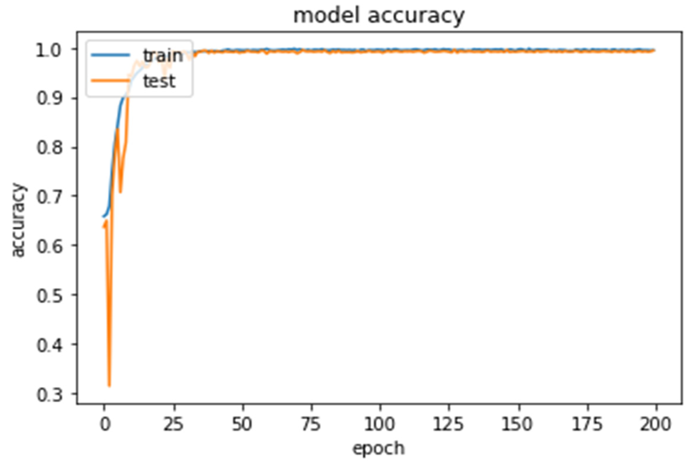
Figure 6 and Figure 7 illustrate the result we obtained from the combination of ReLU activation function and RMSprop optimizer. As anticipated, the higher the training samples and epochs, the lesser the error we achieved. Furthermore, at approximately 200 epochs, its marginal utility diminished, and thus, we made use of only 200 epochs during the experiment. To enhance the classification performance of our model, we deployed less batch size although at the expense of training time. In addition, to smoothen our training iteration and obtain optimal use of GPU, a modest batch size of 32 was used instead of the size of 50 that we originally intended to use although the model experienced some local minima bounce-out due to perturbations emanating from the lesser batch size. The proposed model attained approximately 0.9950 training accuracy and about 0.9943 test accuracy, as shown in

Table 2. The comparisons of the training error and accuracy and test error and accuracy in relation with varying epoch sizes.

RMSprop		Train, Test Accuracy and Loss
Activation	Epochs	Train Error	Train Accuracy	Test Error	Test Accuracy
Scaled Swishmax	50	10.7130	0.3280	10.2327	0.3581
	100	10.4904	0.3420	5.8831	0.3638
	150	10.6216	0.6668	10.1433	0.6374
	200	10.6964	0.3291	10.1212	0.3651
Swishmax	50	5.3677	0.6670	6.0802	0.6228
	100	5.3106	0.6705	5.8831	0.6350
	150	5.3710	0.3337	10.1415	0.3639
	200	5.4130	0.6642	5.8956	0.6342
Leaky Relu	50	5.5456	0.6559	6.2545	0.6120
	100	5.2401	0.6749	5.9939	0.6281
	150	5.2082	0.6769	5.8341	0.6380
	200	5.3996	0.6650	5.7316	0.6444
Prelu	50	0.0166	0.9933	0.0421	0.9873
	100	0.0129	0.9956	0.0438	0.9879
	150	0.0218	0.9931	0.0404	0.9892
	200	0.0122	0.9966	0.0285	0.9924
Relu	50	0.0151	0.9956	0.0506	0.9898
	100	0.0101	0.9966	0.0320	0.9925
	150	0.0155	0.9940	0.0461	0.9917
	200	0.0141	0.9950	0.0266	0.9943

and Figure 8 and Figure 9, respectively. Table 2 illustrates the comparisons of the training error and accuracy and test error and accuracy in relation with varying epoch sizes. The values in bold indicate the best results obtained with RMSprop optimization function with different activation functions, such as scaled swishmax, swishmax, leaky relu, prelu, and relu activation functions

We also experimented with Adam optimizer with varying epochs and different activation functions and L₁ and L₂ reutilization techniques, as shown in

Table 3. The comparisons of the training error and accuracy and test error and accuracy in relation with varying epoch sizes.

Adam		Train, Test Accuracy and Loss
Activation	Epochs	Train Error	Train Accuracy	Test Error	Test Accuracy
$$\begin{gathered} \mathrm{Relu} \\ + \\ {L}_1/L_2 \end{gathered}$$	50	32.6091	0.6492	20.7764	0.6012
	100	40.8956	0.6492	15.8244	0.6411
	150	29.2660	0.6391	19.5986	0.6270
	200	28.1345	0.6411	23.4236	0.6508
Swishmax	50	0.0442	0.9840	0.0527	0.9790
	100	0.0397	0.9877	0.0515	0.9825
	150	0.0408	0.9850	0.0407	0.9854
	200	0.0449	0.9841	0.0541	0.9816
Scaled Swishmax	50	0.0328	0.9861	0.0305	0.9885
	100	0.0341	0.9875	0.0362	0.9875
	150	0.0320	0.9880	0.0307	0.9892
	200	0.0367	0.9843	0.0372	0.9866
Relu	50	0.0279	0.9909	0.0357	0.9879
	100	0.0300	0.9899	0.0361	0.9875
	150	0.0277	0.9891	0.0389	0.9841
	200	0.0245	0.9912	0.0390	0.9873
Prelu	50	0.0256	0.9909	0.0415	0.9930
	100	0.0239	0.9937	0.0368	0.9938
	150	0.0271	0.9922	0.0453	0.9924
	200	0.0274	0.9909	0.0387	0.9930
Leaky Relu	50	0.0098	0.9969	0.0282	0.9924
	100	0.0102	0.9969	0.0237	0.9938
	150	0.0120	0.9956	0.0280	0.9930
	200	0.0108	0.9956	0.0228	0.9936

. The comparisons of the training error and accuracy and test error and accuracy in relation with varying epoch sizes is illustrated in Table 3. The values in bold indicate the best results obtained with Adam optimization function with L₁ and L₂ regularizers and different activation functions, such as scaled swishmax, swishmax, leaky relu, prelu, and relu activation functions.

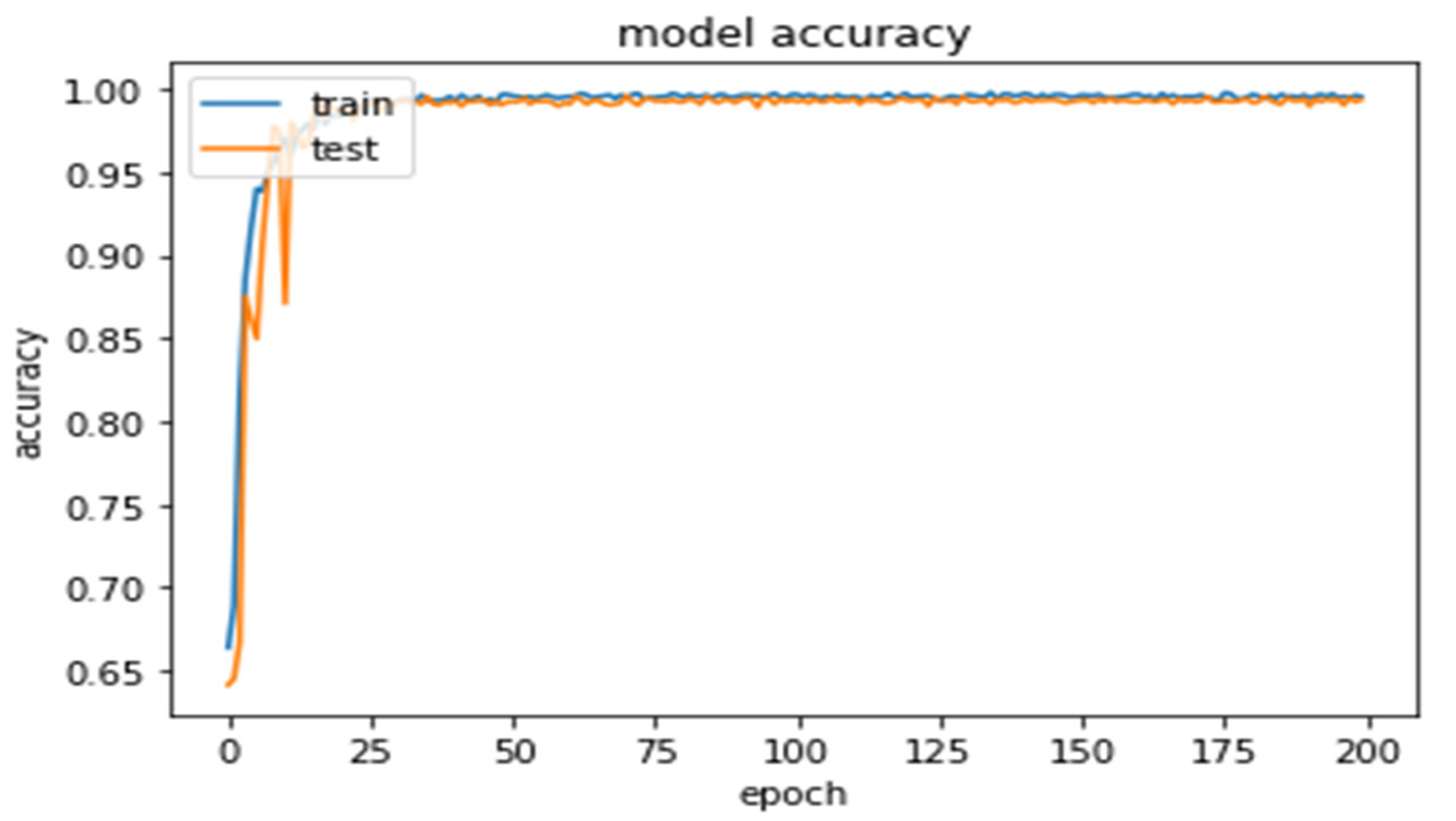
As illustrated in Table 3 and Figure 8 and Figure 9, the validation accuracy and loss between the various activation functions used, except (Relu + $L_1/L_2$), are averagely 0.98842 and 0.038622, respectively, when all the training samples are used. However, the combination of (Relu + $L_1/L_2$) yielded poor performance due to the heavy influence of the regularization terms. This shows that the choice of activation function can, to a large extent, influence the classification performance of a CNN model. Astonishingly, the classification performance differs with varied epochs. To mitigate overfitting when using a small dataset, heavy augmentation techniques are required, and if smaller size of image are used, discriminative information is easily lost during training, thereby affecting the overall performance of the model. Owing to the fixed structure of the model, an insufficient training sample to learn numerous parameters for smaller image samples can lead to overfitting problems.

As shown in Table 2 and Figure 5 and Figure 6, the combination of RMSprop optimization and ReLU activation function produced best validation result and lower classification loss than other activation functions. Our model attained reasonable classification performance, and therefore, it can be established that our model is robust for classifying cracked surface of tiles from no-cracked image samples.

In our effort to enhance the classification accuracy of our model, we modified our network architecture by increasing the size of the convolutional layers, size of learning filters, and introducing combined L₁ and L₂ regularization terms into our network. This in turn increased the architecture’s total parameter from 3,453,121 to 7,146,257, trainable parameters to 7,146,065, and non-trainable parameters to 192.

We recorded perfect learning movement, as shown in Figure 10 and Figure 11, but due to light deployment of data augmentation techniques and insufficient training data, the modified network architecture could not achieve high validation accuracy.

6. Discussion

The comparative study is given in

Table 4. Comparative performances of deep learning-based crack-detection studies.

Methods	Strengths	Weaknesses	Applicable
Crack detection using image processing [92]	To crack classification tasks, Feature Pyramid Network (FPN) approach was adopted to process the outcome of a GoogleNet. The FPN was built up with layers fussed together in conjunction with convolutional layers	Low processing speed of the proposed model. It takes an approximately 16 s to process and detect the entire crack content	6000 × 4000 pixels images.
Pixel-level read crack detection in black-box images [93]	A deep convolutional encoder-decoder network model was utilized to identify road fractures at the pixel level. The suggested model’s encoder component is made up of convolutional layers, which are responsible for extracting crack characteristics. The decoder part is made up of de-convolutional layers, which detect where fractures in picture samples are located.	Quantify the cracks and type of cracks and needs more accurate pixel-level cracks in the road. Need a large-scale image database.	427 black box images were used for the model training and 100 images used for the model testing process.
Crack detection with fully convolutional network [93]	Crack segmentation predictions were represented as pixel skeletons with a width of one pixel, which were then utilized to measure morphological parameters, such as width, length, and topology, in the pictures.	There is no fixed or equivalent bounding box in these circumstances; hence, pixel-level identification is required.	Detect cracks at pixel level
Ceramic defect detection using convolutional neural network (present study)	Uses an in-depth learning-based method rather than a filter-based method. Geometric properties are not dependent. We used the feature and discrimination techniques. Deployed on images that are acquired using low-cost, ordinary smart phone cameras that pose complex features	Detects of surface defects on ceramic tiles only.	Material that is put to the test (ceramic)

. In [91], a Feature Pyramid Network (FPN) approach was adopted to process the outcome of a GoogleNet Convolutional neural network architecture used for the crack-classification tasks. The feature pyramid network was built up with layers fussed together in conjunction with convolutional layers that work collectively to conduct the delineation of crack processes. A precisive accuracy of 80.13% for the crack delineation process was achieved in the work. However, the low processing speed of the proposed model is the major drawback, as it takes approximately 16 s to process and detect the entire crack content of a 6000 × 4000 pixels image.

Ref. [92] used a deep convolutional encoder-decoder network model to perform a pixel-level road-cracks detection. The encoder section of the proposed model is composed of the convolutional layers, which is responsible for the crack features extraction. On the other hand, the decoder section is made up of the de-convolutional layers that determines the locations of cracks in the image samples. In their experiments, 427 black box images were used for the model training and 100 images used for the model testing process. They obtained an intersection of a union score of 59.65%, a recall of 71.98%, and a precision of 77.68%, respectively. In [93], a Fully Convolutional Network (FCN) architecture was utilized to perform the pixel-wise segmentation of cracks that exist in image samples of pavements and walls. In the model, crack segmentation predictions were represented using pixel skeletons with a width of a pixel and the skeletons then used to measure the images’ morphological features, such as width, length, and topology. They obtained an overall accuracy of 97.96%, which is far better than the CrackNet model because the model generates pixel-level segmentation and uses less training time.

Comparing our proposed architecture with the others in the literature, our model ushered in a more accurate, efficient, and less complex architecture for identifying cracks in the tile’s smooth surfaces. The model uses less parameters and in turn is less computationally intensive, which are crucial for the model inferencing and deployment. We achieved an accuracy of 99.43%, which is closely followed by the Yang et al. [93] model at 97.96%. Our proposed model achieved an improvement of 1.47%, which is highly significant in precisive cracks spotting from tile surfaces.

7. Conclusions

In this work, we present a simple CNN model to handle the classification tasks of close, similar defect of smooth tile surface. When compared to the existing methods and classical handcrafted feature-extraction system, our proposed method attains multiple purposes of simultaneous classification and features extraction. The results obtained from our detailed experiments demonstrate the efficiency of our approach with small tile crack and no-crack dataset. With extensive deployment of data augmentation methods on a small training and test dataset, our proposed model is able to realize satisfactory validation accuracy on smooth tile-surface defects, with average classification accuracy of approximately 0.9943 and 0.0266 classification loss on test set. For future work, more types of tile-surface defects from different types of tile surface and designs will be collected and a more robust classifier built.

References

- Jahangiri, A.; Rakha, H.A.; Dingus, T.A. Adopting machine learning methods to predict red-light running violations. In Proceedings of the IEEE International Conference on Intelligent Transportation Systems, Gran Canaria, Spain, 15–18 September 2015; pp. 650–655. [Google Scholar]
- Oliveira, H.; Correia, P.L. CrackIT—An Image Processing Toolbox for Crack Detection and Characterization. In Proceedings of the 2014 IEEE International Conference on Image Processing (ICIP), Paris, France, 27–30 October 2014; pp. 798–802. [Google Scholar] [CrossRef]
- Budiansky, B.; O’Connell, R.J. Elastic moduli of a cracked solid. Int. J. Solids Struct. 1976, 12, 81–97. [Google Scholar] [CrossRef]
- Aboudi, J. Stiffness reduction of cracked solids. Eng. Fract. Mech. 1987, 26, 637–650. [Google Scholar] [CrossRef]
- Lacidogna, G.; Piana, G.; Accornero, F.; Carpinteri, A. Multi-technique damage monitoring of concrete beams: Acoustic Emission, Digital Image Correlation, Dynamic Identification. Constr. Build. Mater. 2020, 242, 118114. [Google Scholar] [CrossRef]
- Zhao, S.; Sun, L.; Gao, J.; Wang, J.; Shen, Y. Uniaxial ACFM detection system for metal crack size estimation using magnetic signature waveform analysis. Measurement 2020, 164, 108090. [Google Scholar] [CrossRef]
- Zhang, X.; Wang, K.; Wang, Y.; Shen, Y.; Hu, H. Rail crack detection using acoustic emission technique by joint optimization noise clustering and time window feature detection. Appl. Acoust. 2019, 160, 107141. [Google Scholar] [CrossRef]
- Cheon, M.H.; Hong, D.G.; Lee, D.H. Surface crack detection in concrete structures using image processing. In Proceedings of the 2017 International Conference on Robot Intelligence Technology and Applications, Daejeon, Korea, 14–15 December 2017. [Google Scholar]
- Zou, Q.; Cao, Y.; Li, Q.; Mao, Q.; Wang, S. CrackTree: Automatic crack detection from pavement images. Pattern Recognit. Lett. 2012, 33, 227–238. [Google Scholar] [CrossRef]
- Mathavan, S.; Kamal, K.; Rahman, M. A Review of Three-Dimensional Imaging Technologies for Pavement Distress Detection and Measurements. IEEE Trans. Intell. Transp. Syst. 2015, 16, 2353–2362. [Google Scholar] [CrossRef] [Green Version]
- Medina, R.; Llamas, J.; Zalama, E.; Gomez-Garcia-Bermejo, J. Enhanced automatic detection of road sur-face cracks by combining 2d/3d image processing techniques. In Proceedings of the IEEE International Conference on Image Processing, Paris, France, 27–30 October 2014; pp. 778–782. [Google Scholar]
- Varadharajan, S.; Jose, S.; Sharma, K.; Wander, L.; Mertz, C. Vision for road inspection. In Proceedings of the 2014 IEEE Winter Conference on Applications of Computer Vision, Steamboat Springs, CO, USA, 24–26 March 2014; pp. 115–122. [Google Scholar]
- Roth, H.R.; Lu, L.; Liu, J.; Yao, J.; Seff, A.; Cherry, K.; Kim, L.; Summers, R.M. Improving Computer-Aided Detection Using_newlineConvolutional Neural Networks and Random View Aggregation. IEEE Trans. Med. Imaging 2015, 35, 1170–1181. [Google Scholar] [CrossRef] [Green Version]
- Kivinen, J.J.; Williams, C.K.; Heess, N. Visual boundary prediction: A deep neural prediction network and quality dissection. In Proceedings of the International Conference on Artificial Intelligence and Statistics, Reykjavik, Iceland, 22–25 April 2014; pp. 512–521. [Google Scholar]
- LeCun, Y.; Bengio, Y.; Hinton, G. Deep learning. Nature 2015, 521, 436–444. [Google Scholar] [CrossRef] [PubMed]
- Cho, K. Boltzmann Machines for Image Denoising. In Artificial Neural Networks and Machine Learning—ICANN 2013; Lecture Notes in Computer Science; Mladenov, V., Koprinkova-Hristova, P., Palm, G., Villa, A.E.P., Appollini, B., Kasabov, N., Eds.; Springer: Berlin/Heidelberg, Germany, 2013; pp. 611–618. [Google Scholar] [CrossRef]
- Deng, L.; Seltzer, M.L.; Yu, D.; Acero, A.; Mohamed, A.R.; Hinton, G. Binary Coding of Speech Spectrograms Using a Deep Auto-Encoder. In Proceedings of the Eleventh Annual Conference of the International SPEECH communication Association, Makuhari, Chiba, Japan, 26–30 September 2010; pp. 1692–1695. [Google Scholar]
- Salman, M.; Mathavan, S.; Kamal, K.; Rahman, M. Pavement crack detection using the gabor filter. In Proceedings of the IEEE International Conference on Intelligent Transportation Systems, The Hague, The Netherlands, 6–9 October 2013; pp. 2039–2044. [Google Scholar]
- Hu, Y.; Zhao, C. A local binary pattern-based methods for pavement crack detection. J. Pattern Recognit. Res. 2010, 5, 140–147. [Google Scholar] [CrossRef]
- Oliveira, H.; Correia, P.L. Automatic road crack detection and characterization. IEEE Trans. Intell. Transp. Syst. 2013, 14, 155–168. [Google Scholar] [CrossRef]
- Abdel-Qader, I.; Abudayyeh, O.; Kelly, M.E. Analysis of Edge-Detection Techniques for Crack Identification in Bridges. J. Comput. Civ. Eng. 2003, 17, 255–263. [Google Scholar] [CrossRef]
- Fujita, Y.; Hamamoto, Y. A robust automatic crack detection method from noisy concrete surfaces. Mach. Vis. Appl. 2011, 22, 245–254. [Google Scholar] [CrossRef]
- Jahanshahi, M.R.; Masri, S.F. Adaptive vision-based crack detection using 3D scene reconstruction for condition assessment of structures. Autom. Constr. 2012, 22, 567–576. [Google Scholar] [CrossRef]
- Chen, F.-C.; Jahanshahi, M.R.; Wu, R.-T.; Joffe, C. A texture-Based Video Processing Methodology Using Bayesian Data Fusion for Autonomous Crack Detection on Metallic Surfaces. Comput. Civ. Infrastruct. Eng. 2017, 32, 271–287. [Google Scholar] [CrossRef]
- Dung, C.V.; Anh, L.D. Autonomous concrete crack detection using deep fully convolutional neural network. Autom. Constr. 2018, 99, 52–58. [Google Scholar] [CrossRef]
- Yamaguchi, T.; Hashimoto, S. Fast crack detection method for large-size concrete surface images using percolation-based image processing. Mach. Vis. Appl. 2009, 21, 797–809. [Google Scholar] [CrossRef]
- Bu, P.; Chanda, S.; Guan, H.; Jo, J.; Blumenstein, M.; Loo, Y.C. Crack detection using a texture analysis-based technique for visual bridge inspection. Electron. J. Struct. Eng. 2015, 14, 41–48. [Google Scholar]
- Jahanshahi, M.R.; Masri, S.F.; Padgett, C.W.; Sukhatme, G.S. An innovative methodology for detection and quantification of cracks through incorporation of depth perception. Mach. Vis. Appl. 2013, 24, 227–241. [Google Scholar] [CrossRef]
- Zalama, E.; Gómez-García-Bermejo, J.; Medina, R.; Llamas, J. Road crack detection using visual features extracted by gabor filters. Comput. Aided Civ. Infrastruct. Eng. 2014, 29, 342–358. [Google Scholar] [CrossRef]
- Wu, X.-Y.; Xu, K.; Xu, J.-W. Application of un-decimated wavelet transform to surface defect detection of hot rolled steel plates. Proc. Congr. Image Signal Process. 2008, 4, 528–532. [Google Scholar]
- Choi, D.-C.; Jeon, Y.-J.; Lee, S.J.; Yun, J.P.; Kim, S.W. Algorithm for detecting seam cracks in steel plates using a Gabor filter combination method. Appl. Opt. 2014, 53, 4865–4872. [Google Scholar] [CrossRef] [PubMed]
- Zou, Q.; Zhang, Z.; Li, Q.; Qi, X.; Wang, Q.; Wang, S. DeepCrack: Learning Hierarchical Convolutional Features for Crack Detection. IEEE Trans. Image Process. 2019, 28, 1498–1512. [Google Scholar] [CrossRef] [PubMed]
- Schmugge, S.J.; Nguyen, N.R.; Thao, C.; Lindberg, J.; Grizzi, R.; Joffe, C.; Shin, M.C. Automatic detection of cracks during power plant inspection. In Proceedings of the 2014 3rd International Conference on Applied Robotics for the Power Industry, Foz do Iguacu, Brazil, 14–16 October 2014; pp. 1–5. [Google Scholar] [CrossRef]
- Lundervold, A.S.; Lundervold, A. An overview of deep learning in medical imaging focusing on MRI. Z. Med. Physik 2019, 29, 102–127. [Google Scholar] [CrossRef]
- Yin, S.; Luo, H.; Ding, S.X. Real-Time Implementation of Fault-Tolerant Control Systems with Performance Optimization. IEEE Trans. Ind. Electron. 2013, 61, 2402–2411. [Google Scholar] [CrossRef]
- Yin, S.; Yang, H.; Gao, H.; Qiu, J.; Kaynak, O. An Adaptive NN-Based Approach for Fault-Tolerant Control of Nonlinear Time-Varying Delay Systems with Unmodeled Dynamics. IEEE Trans. Neural Netw. Learn. Syst. 2016, 28, 1902–1913. [Google Scholar] [CrossRef]
- Alzubaidi, L.; Zhang, J.; Humaidi, A.J. Review of deep learning: Concepts, CNN architectures, challenges, applications, future directions. J. Big Data 2021, 8, 53. [Google Scholar] [CrossRef]
- Deng, J.; Dong, W.; Socher, R.; Li, L.-J.; Li, K.; Fei-Fei, L. ImageNet: A large-scale hierarchical image database. In Proceedings of the 2009 IEEE Conference on Computer Vision and Pattern Recognition, Miami, FL, USA, 20–25 June 2009; pp. 248–255. [Google Scholar]
- Girshick, R.; Donahue, J.; Darrell, T.; Malik, J. Richfeaturehierarchies for accurate object detection and semantic segmentation. In Proceedings of the IEEE Conference on Computer Vision and Pattern Recognition, Columbus, OH, USA, 23–28 June 2014; pp. 580–587. [Google Scholar]
- Girshick, R. Fast R-CNN. In Proceedings of the IEEE International Conference on Computer Vision (ICCV), Sydney, Australia, 7–13 December 2015; pp. 1440–1448. [Google Scholar]
- Ren, S.; He, K.; Girshick, R.; Sun, J. Faster R-CNN: Towards real-time object detection with region proposal networks. Adv. Neural Inf. Process. Syst. 2015, 28, 91–99. [Google Scholar] [CrossRef] [Green Version]
- Zhang, L.; Yang, F.; Zhang, Y.D.; Zhu, Y.J. Road crack detection using deep convolutional neural network. In Proceedings of the International Conference on Image Processing, ICIP, Phoenix, AZ, USA, 25–28 September 2016; pp. 3708–3712. [Google Scholar] [CrossRef]
- Cha, Y.-J.; Choi, W.; Büyüköztürk, O. Deep learning-based crack damage detection using convolutional neural networks. Comput.-Aided Civ. Infrastruct. Eng. 2017, 32, 361–378. [Google Scholar] [CrossRef]
- Schmugge, S.J.; Rice, L.; Nguyen, N.R.; Lindberg, J.; Grizzi, R.; Joffe, C.; Shin, M.C. Detection of cracks in nuclear power plant using spatial-temporal grouping of local patches. In Proceedings of the 2016 IEEE Winter Conference on Applications of Computer Vision (WACV), Lake Placid, NY, USA, 7–10 March 2016; pp. 1–7. [Google Scholar] [CrossRef]
- Soukup, D.; Huber-Mörk, R. Convolutional neural networks for steel surface defect detection from photometric stereo images. In Proceedings of the International Symposium on Visual Computing, Tokyo, Japan, 8–9 May 2014; pp. 668–677. [Google Scholar]
- Zhang, A.; Wang, K.C.P.; Fei, Y.; Liu, Y.; Tao, S.; Chen, C.; Li, J.Q.; Li, B. Deep Learning—Based Fully Automated Pavement Crack Detection on 3D Asphalt Surfaces with an Improved CrackNet. J. Comput. Civ. Eng. 2018, 32, 04018041. [Google Scholar] [CrossRef] [Green Version]
- Pauly, L.; Hogg, D.; Fuentes, R.; Peel, H. Deeper networks for pavement crack detectionIAARC. In Proceedings of the 34th International Symposium on Automation and Robotics in Construction and Mining (ISARC 2017), Taipei, Taiwan, 28 June–1 July 2017. [Google Scholar]
- Agarap, A.F. Deep learning using rectified linear units (relu). arXiv 2018, arXiv:1803.08375. [Google Scholar]
- Yang, H.; Yu, L. Feature extraction of wood-hole defects using wavelet-based ultrasonic testing. J. For. Res. 2017, 28, 395–402. [Google Scholar] [CrossRef]
- Shanmugamani, R.; Sadique, M.; Ramamoorthy, B. Detection and classification of surface defects of gun barrels using computer vision and machine learning. Measurement 2015, 60, 222–230. [Google Scholar] [CrossRef]
- Gholizadeh, S.; Leman, Z.; Baharudin, B. A review of the application of acoustic emission technique in engineering. Struct. Eng. Mech. 2015, 54, 1075–1095. [Google Scholar] [CrossRef]
- Rocha, T.; Ramos, H.G.; Ribeiro, A.; Pasadas, D.J. Magnetic sensors assessment in velocity induced eddy current testing. Sens. Actuators A Phys. 2015, 228, 55–61. [Google Scholar] [CrossRef]
- Lecun, Y.; Bottou, L.; Bengio, Y.; Haffner, P. Gradient-based learning applied to document recognition. Proc. IEEE 1998, 86, 2278–2324. [Google Scholar] [CrossRef] [Green Version]
- Lee, Y.H. Efficiency Improvement in a Busy Radiology Practice: Determination of Musculoskeletal Magnetic Resonance Imaging Protocol Using Deep-Learning Convolutional Neural Networks. J. Digit. Imaging 2018, 31, 604–610. [Google Scholar] [CrossRef] [PubMed]
- Gong, E.; Pauly, J.M.; Wintermark, M.; Zaharchuk, G. Deep learning enables reduced gadolinium dose for contrast-enhanced brain MRI. J. Magn. Reson. Imaging 2018, 48, 330–340. [Google Scholar] [CrossRef]
- Liu, F.; Jang, H.; Kijowski, R.; Bradshaw, T.; McMillan, A.B. Deep Learning MR Imaging–based Attenuation Correction for PET/MR Imaging. Radiology 2018, 286, 676–684. [Google Scholar] [CrossRef]
- Meyer, P.; Noblet, V.; Mazzara, C.; Lallement, A. Survey on deep learning for radiotherapy. Comput. Biol. Med. 2018, 98, 126–146. [Google Scholar] [CrossRef] [PubMed]
- Lee, J.-G.; Jun, S.; Cho, Y.-W.; Lee, H.; Kim, G.B.; Seo, J.B.; Kim, N. Deep Learning in Medical Imaging: General Overview. Korean J. Radiol. 2017, 18, 570–584. [Google Scholar] [CrossRef] [Green Version]
- Rueckert, D.; Glocker, B.; Kainz, B. Learning clinically useful information from images: Past, present and future. Med. Image Anal. 2016, 33, 13–18. [Google Scholar] [CrossRef] [Green Version]
- Chartrand, G.; Cheng, P.M.; Vorontsov, E.; Drozdzal, M.; Turcotte, S.; Pal, C.J.; Kadoury, S.; Tang, A. Deep Learning: A Primer for Radiologists. RadioGraphics 2017, 37, 2113–2131. [Google Scholar] [CrossRef] [PubMed] [Green Version]
- Erickson, B.J.; Korfiatis, P.; Akkus, Z.; Kline, T.L. Machine Learning for Medical Imaging. RadioGraphics 2017, 37, 505–515. [Google Scholar] [CrossRef] [PubMed]
- Mazurowski, M.A.; Buda, M.; Saha, A.; Bashir, M.R. Deep learning in radiology: An overview of the concepts and a survey of the state of the art with focus on MRI. J. Magn. Reson. Imaging 2018, 49, 939–954. [Google Scholar] [CrossRef] [PubMed]
- McBee, M.P.; Awan, O.A.; Colucci, A.T.; Ghobadi, C.W.; Kadom, N.; Kansagra, A.P.; Auffermann, W.F. Deep Learning in Radiology. Acad. Radiol. 2018, 25, 1472–1480. [Google Scholar] [CrossRef] [PubMed] [Green Version]
- Savadjiev, P.; Chong, J.; Dohan, A.; Vakalopoulou, M.; Reinhold, C.; Paragios, N.; Gallix, B. Demystification of AI-driven medical image interpretation: Past, present and future. Eur. Radiol. 2019, 29, 1616–1624. [Google Scholar] [CrossRef]
- Thrall, J.H.; Li, X.; Li, Q.; Cruz, C.; Do, S.; Dreyer, K.; Brink, J. Artificial intelligence and machine learning in radiology: Opportunities, challenges, pitfalls, and criteria for success. J. Am. Coll. Radiol. 2018, 15, 504–508. [Google Scholar] [CrossRef]
- Yamashita, R.; Nishio, M.; Do, R.K.G.; Togashi, K. Convolutional neural networks: An overview and application in radiology. Insights Imaging 2018, 9, 611–629. [Google Scholar] [CrossRef] [PubMed] [Green Version]
- Yasaka, K.; Akai, H.; Kunimatsu, A.; Kiryu, S.; Abe, O. Deep learning with convolutional neural network in radiology. Jpn. J. Radiol. 2018, 36, 257–272. [Google Scholar] [CrossRef]
- Sze, V.; Chen, Y.; Emer, J. Efficient Processing of Deep Neural Networks: A Tutorial and Survey. arXiv 2017, arXiv:1703.09039v2. [Google Scholar] [CrossRef] [Green Version]
- Levine, S.; Finn, C.; Darrell, T.; Abbeel, P. End-to-end training of deep visuomotor policies. J. Mach. Learn. Res. 2016, 17, 1334–1373. [Google Scholar]
- Dvornik, N.; Shmelkov, K.; Mairal, J.; Schmid, C. Blitznet: A real-time deep network for scene understanding. In Proceedings of the IEEE International Conference on Computer Vision (ICCV), Venice, Italy, 22–29 October 2017. [Google Scholar]
- Husain, F.; Dellen, B.; Torras, C. Scene Understanding Using Deep Learning. In Handbook of Neural Computation; Samui, P., Sekhar, S., Balas, V.E., Eds.; Academic Press: Cambridge, MA, USA, 2017; pp. 373–382. ISBN 9780128113189. [Google Scholar] [CrossRef] [Green Version]
- Silver, D.; Huang, A.; Maddison, C.J.; Guez, A.; Sifre, L.; van den Driessche, G.; Schrittwieser, J.; Antonoglou, I.; Panneershelvam, V.; Lanctot, M.; et al. Mastering the game of Go with deep neural networks and tree search. Nature 2016, 529, 484–489. [Google Scholar] [CrossRef]
- He, K.M.; Zhang, X.Y.; Ren, S.Q.; Sun, J. Deep Residual Learning for Image Recognition. In Proceedings of the IEEE Conference on Computer Vision and Pattern Recognition, Las Vegas, NV, USA, 27–30 June 2016; pp. 770–778. [Google Scholar] [CrossRef] [Green Version]
- Nair, V.; Hinton, G.E. Rectified Linear Units Improve Restricted Boltzmann Machines. In Proceedings of the 27th International Conference on Machine Learning (ICML-10), Haifa, Israel, 21–24 June 2010. [Google Scholar]
- He, K.; Zhang, X.; Ren, S.; Sun, J. Delving Deep into Rectifiers: Surpassing Human-Level Performance on ImageNet Classification. In Proceedings of the IEEE International Conference on Computer Vision, Santiago, Chile, 7–13 December 2015; pp. 1026–1034. [Google Scholar] [CrossRef] [Green Version]
- Clevert, D.-A.; Unterthiner, T.; Hochreiter, S. Fast and Accurate Deep Network Learning by Exponential Linear Units (ELUs). arXiv 2015, arXiv:1511.07289. [Google Scholar]
- Maas, A.L.; Hannun, A.Y.; Ng, A.Y. Rectifier Nonlinearities Improve Neural Network Acoustic Models; ICML: Stanford, CA, USA, 2013. [Google Scholar]
- Zhang, X.; Trmal, J.; Povey, D.; Khudanpur, S. Improving deep neural network acoustic models using generalized maxout networks. In Proceedings of the 2014 IEEE International Conference on Acoustics, Speech and Signal Processing (ICASSP), Florence, Italy, 4–9 May 2014; pp. 215–219. [Google Scholar] [CrossRef]
- Zhang, Y.; Pezeshki, M.; Brakel, P.; Zhang, S.; Laurent, C.; Bengio, Y.; Courville, A. Towards End-to-End Speech Recognition with Deep Convolutional Neural Networks. arXiv 2016, arXiv:1701.02720. [Google Scholar] [CrossRef] [Green Version]
- Candes, E.; Tao, T. The Dantzig selector: Statistical estimation when p is much larger than n. Ann. Stat. 2007, 35, 2313–2351. [Google Scholar] [CrossRef] [Green Version]
- ZongBen, X.; Hai, Z.; Yao, W.; Yong, C.X.L. L_(1/2) regularization. Sci. China 2010, 53, 1159–1169. [Google Scholar]
- Tibshirani, R. Regression shrinkage and selection via the Lasso. J. R. Stat. Soc. B 1996, 58, 267–288. [Google Scholar] [CrossRef]
- Fan, J.; Heng, P. Nonconcave penalty likelihood with a diverging number of parameters. Ann. Stat. 2004, 32, 928961. [Google Scholar] [CrossRef] [Green Version]
- Zou, H.; Hastie, T. Regularization and variable selection via the elastic net. J. R. Stat. Soc. B 2005, 67, 301320. [Google Scholar]
- Zou, H. The adaptive Lasso and its oracle properties. J. Am. Stat. Assoc. 2006, 101, 1418–1429. [Google Scholar] [CrossRef] [Green Version]
- Zhao, P.; Yu, B. Stagewise Lasso. J. Mach. Learn. Res. 2007, 8, 2701–2726. [Google Scholar]
- Krizhevsky, A.; Sutskever, I.; Hinton, G.E. ImageNet classification with deep convolutional neural networks. Commun. ACM 2017, 60, 84–90. [Google Scholar] [CrossRef]
- Szegedy, C.; Liu, W.; Jia, Y.; Sermanet, P.; Reed, S.; Anguelov, D.; Erhan, D.; Vanhoucke, V.; Rabinovich, A. Going deeper with convolutions. In Proceedings of the 2015 IEEE Conference on Computer Vision and Pattern Recognition (CVPR), Boston, MA, USA, 7–12 June 2015. [Google Scholar]
- Jarrett, K.; Kavukcuoglu, K.; Ranzato, M.A.; LeCun, Y. What is the best multi-stage architecture for object recognition? In Proceedings of the 2009 IEEE 12th International Conference on Computer Vision, Kyoto, Japan, 29 September–2 October 2009; pp. 2146–2153. [Google Scholar] [CrossRef] [Green Version]
- Available online: http://www.nvidia.com/content/geforce-gtx/NVIDIA_TITAN_Xp_User_Guide.pdf (accessed on 20 August 2021).
- Mohan, A.; Poobal, S. Crack detection using image processing: A critical review and analysis. Alex. Eng. J. 2018, 57, 787–798. [Google Scholar] [CrossRef]
- Bang, S.; Park, S.; Kim, H.; Kim, H. Encoder–decoder network for pixel-level road crack detection in black-box images. Comput.-Aided Civ. Infrastruct. Eng. 2019, 34, 713–727. [Google Scholar] [CrossRef]
- Yang, X.; Li, H.; Yu, Y.; Luo, X.; Huang, T.; Yang, X. Automatic Pixel-Level Crack Detection and Measurement Using Fully Convolutional Network. Comput.-Aided Civ. Infrastruct. Eng. 2018, 33, 1090–1109. [Google Scholar] [CrossRef]
Figure 1.
Proposed network architecture.
Figure 2.
Examples of Activation Functions.
Figure 3.
Two most popular pooling methods.
Figure 4.
A two-layer Neural Network.
Figure 5.
Left, Tile Sample with Crack; Right, Tile Sample without Crack.
Figure 6.
Model’s training and test accuracy over epochs with RMSprop and ReLU.
Figure 7.
Model’s training and test loss over epochs with RMSprop and ReLU.
Figure 8.
Model’s training and test accuracy Adam and LeakyReLU.
Figure 9.
Model’s training and test loss over epochs with Adam and LeakyReLU.
Figure 10.
Model’s training and test accuracy with increased architecture.
Figure 11.
Model’s training and test loss with increased architecture.