Article

Non-Contact Crack Visual Measurement System Combining Improved U-Net Algorithm and Canny Edge Detection Method with Laser Rangefinder and Camera

1
School of Hydraulic Engineering, Faculty of Infrastructure Engineering, Dalian University of Technology, Dalian 116024, China
2
College of Water Conservancy and Hydropower Engineering, Hohai University, Nanjing 210098, China
*
Authors to whom correspondence should be addressed.
Appl. Sci. 2022, 12(20), 10651; https://doi.org/10.3390/app122010651
Submission received: 28 September 2022 / Revised: 12 October 2022 / Accepted: 17 October 2022 / Published: 21 October 2022
(This article belongs to the Special Issue Machine Learning–Based Structural Health Monitoring)

Abstract

:
Cracks are the main damages of concrete structures. Since cracks may occur in areas that are difficult to reach, non-contact measurement technology is required to accurately measure the width of cracks. This study presents an innovative computer vision system combining a camera and laser rangefinder to measure crack width from any angle and at a long distance. To solve the problem of pixel distortion caused by non-vertical photographing, geometric transformation formulas that can calculate the unit pixel length of the image captured at any angle are proposed. The complexity of crack edge calculation and the imbalance of data in the image are other problems that affect measurement accuracy, and a combination of the improved U-net convolutional networks algorithm and Canny edge detection method is adopted to accurately extract the cracks. The measurement results on the different concrete wall indicate that the proposed system can measure the crack in a non-vertical position, and the proposed algorithm can extract the crack from different background images. Although the proposed system cannot achieve fully automated measurement, the results also confirm the ability to obtain the crack width accurately and conveniently.

1. Introduction

The occurrence of cracks is one of the most common damages to a concrete surface and the earliest form of structural failure. The patterns and scales of cracks may reveal the health conditions and damage levels of concrete structures [1]. The widely adopted methods for crack detection include periodic visual inspections, which are inaccurate, expensive, subjective and labor-intensive [2]. Furthermore, because there are many locations on the large structures, such as the bottom of a bridge or spillway of dams, it is often difficult for inspectors to reach the locations, and this renders the monitoring of the cracks for a long period challenging. Over the past decades, many researchers have analyzed the materials using excellent algorithms, have paid attention to numerical simulation schemes to measure the scale and development trend of structural damages [3,4] or have applied nonlinear analysis to cross-scale modeling to ensure safety [5,6]. These methods are usually based on existing data for analysis. However, the previously arranged sensors cannot cover new cracks, and it is inconvenient for new contact sensors to be installed on the structural surfaces. Therefore, a non-contact accurate measurement method is needed to measure concrete cracks.
With the development of computer vision technology, many crack detection algorithms have been proposed. The traditional crack detection method is the Canny algorithm based on computing digital gradients [7]. However, due to the complex background, the edges of the cracks cannot be uniquely extracted. In recent years, damage identification and concrete structural analysis methods using deep learning with convolutional neural networks (CNN) or artificial intelligence methods have been widely adopted [8]. Deep learning methods have significant advantages compared to traditional image processing techniques or other machine learning techniques [9]. As multilevel features of damages are extracted from the images, deep learning can automatically learn data and update internal parameters continuously to achieve automatic recognition. Deep learning methods have been widely applied for structural health monitoring and are mainly divided into two approaches: object detection and image segmentation based on region division [10]. Considering the patterns of cracks, segmentation methods based on deep learning are suitable for accurately extracting and measuring cracks. The CNN model combined with a sliding window was adopted by Cha to detect cracks on concrete surfaces [9], and the results proved that the deep learning method can extract cracks accurately. To simplify the implementation process and classify the images at the pixel level, an end-to-end architecture based on a fully convolutional neural network (FCN) was conceived [11]. Dung presented the FCN for crack detection, and not only were the cracks reasonably detected but the density was also accurately evaluated [12]. Yang showed the reduced training time of FCN, feeding the train model with 224 × 224 size images [13]. Since the image training size can affect the results, the crop size should be carefully considered according to the actual image. There are large numbers of other crack segmentation algorithms based on deep learning that have been proposed [14], and these studies have proven the broad applicability of deep learning.
The U-net architecture based on FCN was created by Ronneberger and has become a classical semantic segmentation method [15]. Liu found that the U-net model shows higher accuracy for crack segmentation by examining the fundamental parameters representing the performance of the method, proving that the algorithm can be widely adopted for non-contact measurement [10]. Chen extracted cracks with the combination of CNN classification and U-net segmentation and improved the reliability and efficiency of detecting and differentiating facade cracks from complicated facade noises [16]. To train the model more efficiently and obtain higher accuracy, many studies have chosen to improve the U-net model. Aslam used a supervised learning approach to inspect defects from digital images of titanium-coated metal surfaces [17]. Zhang improved the U-net model based on a new loss function named generalized dice loss to detect cracks more accurately, which indicated that a different loss function can affect segmentation results [11]. Sajedi combined the underlying idea of U-net with other networks to achieve urban scene segmentation, resulting in a new approach for the improvement of the network [18]. With a comprehensive crack detection system, real-world images demonstrate that the U-net method can quantify various cracks accurately and robustly [19]. Although the accuracy and various evaluation indicators demonstrate the practicality of deep learning in crack segmentation, there are fewer definitions of the boundaries of the crack in dataset or extraction results, and measurement errors may result.
After accurately extracting the crack pixels, many scholars apply the results in many fields. In recent years, vision-based sensors have been confirmed as a practical method for non-contact and accurate measurement, in which distances are extracted by calculating the distances or moving positions of the pixel-grids [20]. For small-scale concrete structures, many experiments have proven the feasibility of machine vision in crack detection. Jiang [21] proposed a real-time crack inspection method with a wall-climbing unmanned aerial system, calculating the crack width at fixed distance. Dias [22] adopted photogrammetry to extract global crack maps from the surface of the structure, and the universality of the digital image correlation approach was proven. For non-planar structures, 3D digital image correlation systems were used to analyze the compression behavior of concrete structures during deformation [23,24,25]. Machine vision technology is also applied to the detection of structural cracks or other related issues [26,27]. Ji [28] developed a vision-based measurement method for experimental tests of reinforced concrete structures, which can measure deformations and characterize cracks from images of specimens. Valenca [29] designed a method based on image processing to automatically monitor cracks in concrete dams, and the results validate the ability of computer vision to perform a detailed characterization of cracks in concrete dams.
The purpose of this study is to realize the long distance and non-contact precise measurement of the crack width through computer vision. A combination system with a camera and laser rangefinder is proposed as measurement equipment. To solve the problem of pixel distortion caused by non-vertical photographing, the innovative geometric transformation formulas are proposed, which can calculate the unit pixel length of the target plane image captured at any angle. To solve the data imbalance problem caused by a smaller crack pixel proportion, the improved U-net algorithm is proposed to accurately segment the crack areas, and the Canny edge detection method is adopted to refine the edge and ensure that it follows mathematical standards. Errors of measuring equipment, systems and segmentation algorithms are analyzed by standard size targets and artificial cracks. The performances of the crack measurement system are tested on a real wall in the lab and applied to some cracks with different backgrounds on a concrete dam. The object is to propose a practical system to measure the crack width by simple steps, and the equipment can be moved to measure sudden cracks or fixed to monitor the change of cracks for a long time.
The rest of the paper is organized as follows: Section 2 describes the problem of crack detection based on computer vision, Section 3 proposes the geometric model of the combination of the camera and laser rangefinder system and the crack extraction process based on improved U-net segmentation, Section 4 validates the method on the real concrete wall, and Section 5 draws the conclusion.

2. The Problem of Crack Measurement Based on Machine Vision

2.1. Computer Vision-Based Measurement System

Various measurement models based on computer vision have been proposed to detect cracks [30]. Camera imaging models are usually separated into two kinds: the simple pinhole camera model and Gauss camera imaging model. The Gauss camera imaging model is the most suitable model for engineering projects due to the suitable camera focusing expression, and the imaging geometrical relationship of Gauss model is shown in Figure 1. If an object with length L m is on the target plane, the projection length on the image plane would be S pixels. The distance between the target plane and optical center O is object distance U and usually can be calculated by a laser rangefinder. Image distance V represents the relationship of optical center O and the sensor plane, which is usually small, and the value will be affected by the focusing operation of the digital camera. Each point on the target plane will emit two rays: one passes through optical center O in a straight direction, with the other parallel to the optical axis, refracted by the camera lens, and intersecting with the first ray on the imaging plane. Focal length f is the distance between optical center O and the intersection of the second ray and optical axis. The geometric relation between focal length f, object distance U and image distance V can be described using Equation (1).
1 U + 1 V = 1 f ,
where the object distance U can be obtained by measuring equipment, and the focal length f is related to lens selection. The image distance V is calculated as Equation (2).
V = U f U f ,
When the captured image is clear, the image distance is automatically adjusted according to other variables. The pixel length S can be calculated by the pixel number pix and unit pixel size ε as shown in Equation (3).
S = p i x ε ,
If the camera optical axis is perpendicular to the object plane, according to the principle of triangulation, the actual physical width L can be described by the pixel length S as Equation (4).
L U = S V L = S U V = p i x × ε ( U f ) f ,
Although the imaging formula can be used to represent the object width by measuring the object distance U and pixel length S, there are many problems that can affect the precision and result of converting a pixel to the actual length. As the adopted Gauss model is idealized and not applicable in practice, there are three main problems.
(1)
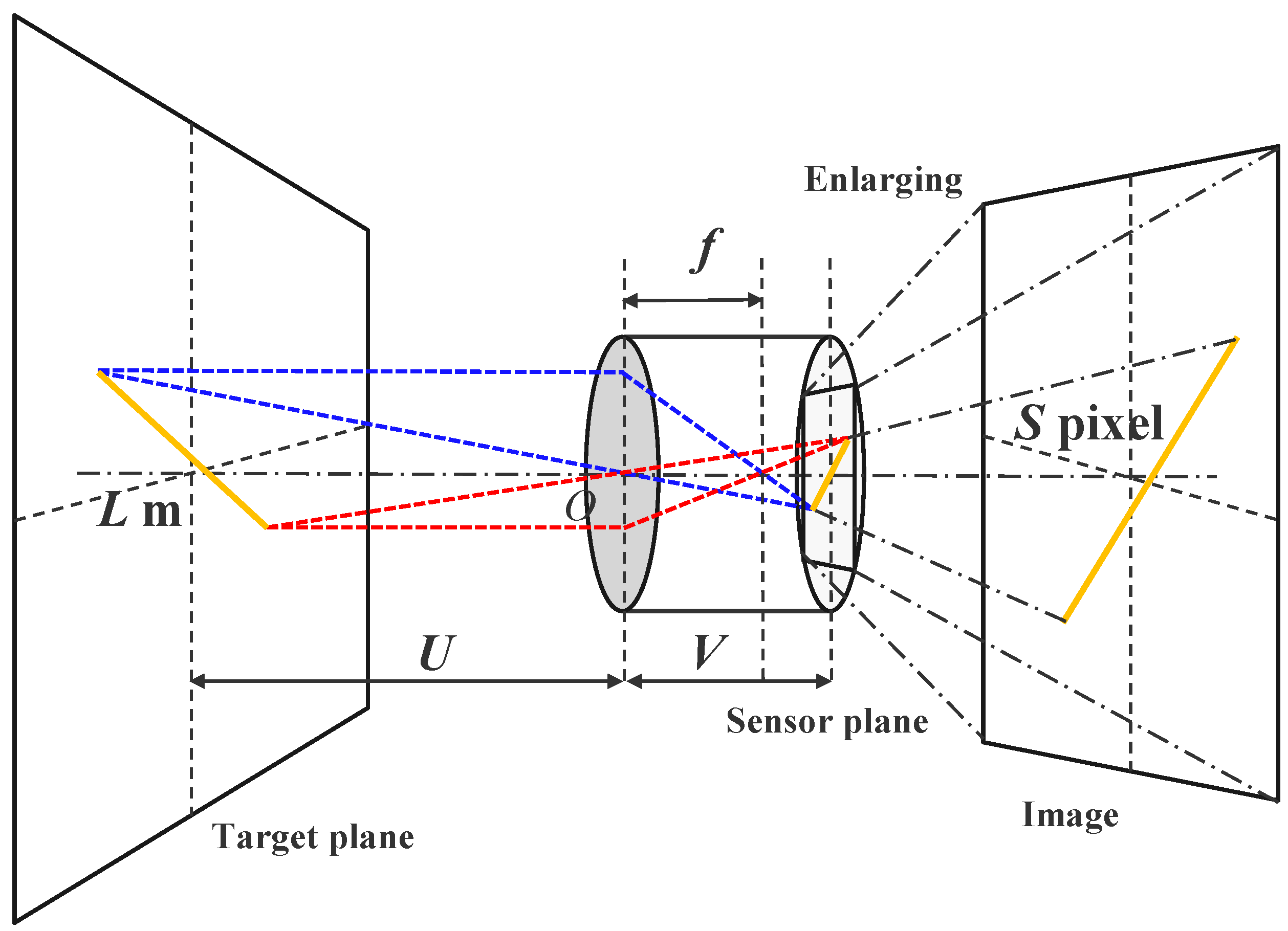
Theoretically, the object distance is the space from the center of the lens O to the object surface, which is hard to accurately acquire and will cause the error in Equation (4). Moreover, the common range of focal length f is usually from 0.018 m to 0.2 m, while the error is usually at the centimeter scale; it can be seen that the lower the focal length f, the larger the impact, resulting in an unignorable error.
(2)
Digital cameras are divided into half and full frame types, and the focal length f is usually obtained manually. However, the manual focal length f is different from that in the Gaussian model and should be corrected before measuring, which may cause an incorrect physical width L in Equation (4).
(3)
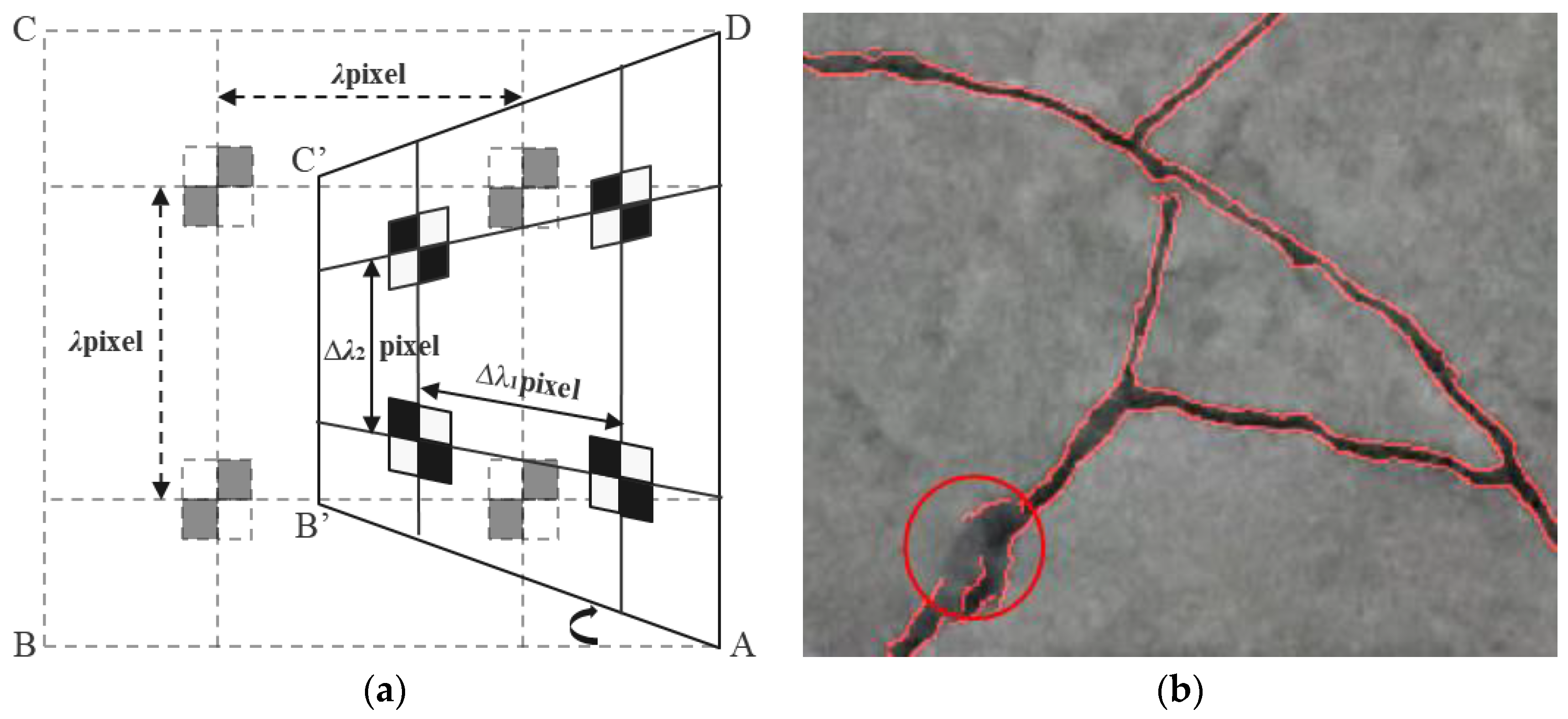
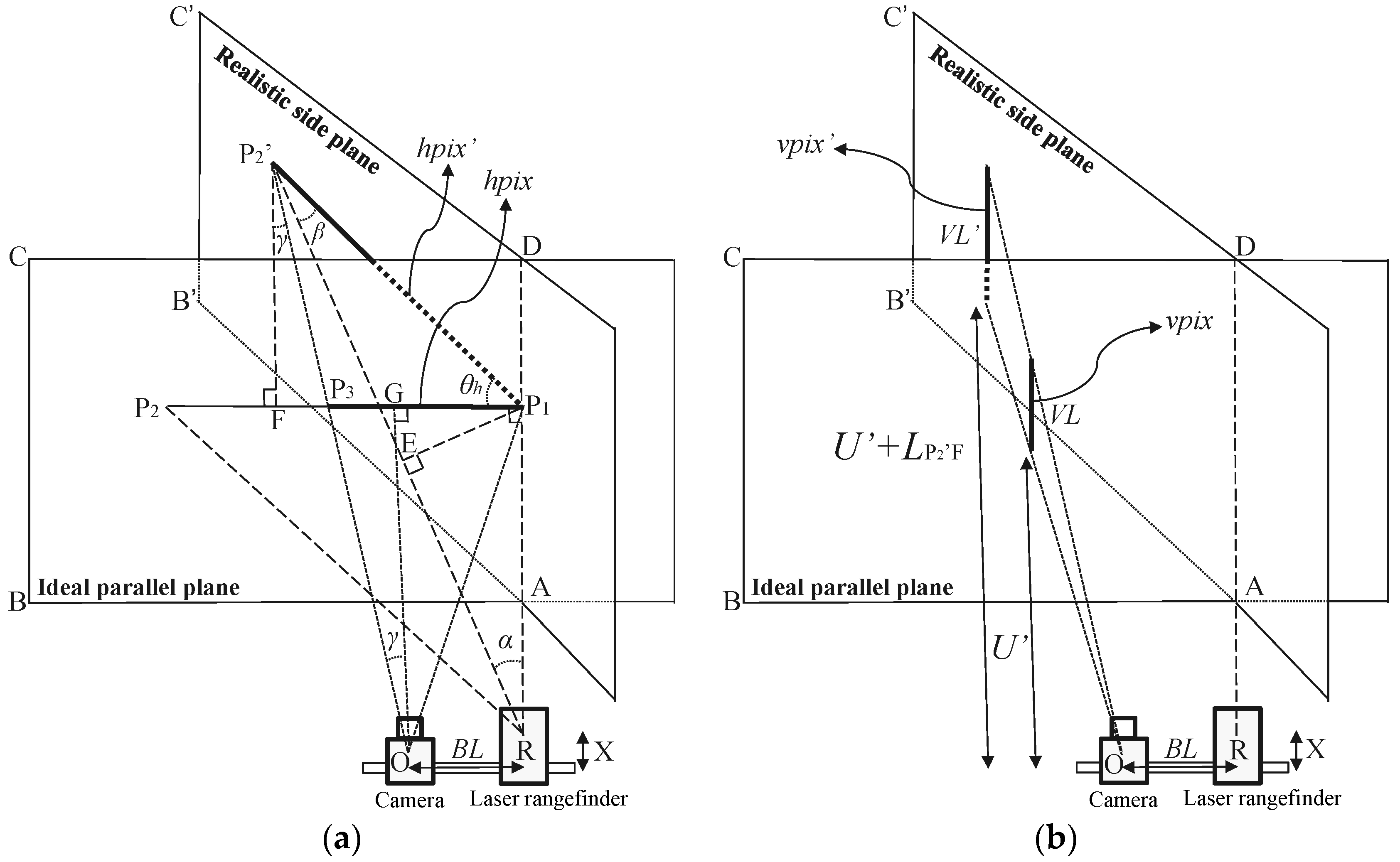
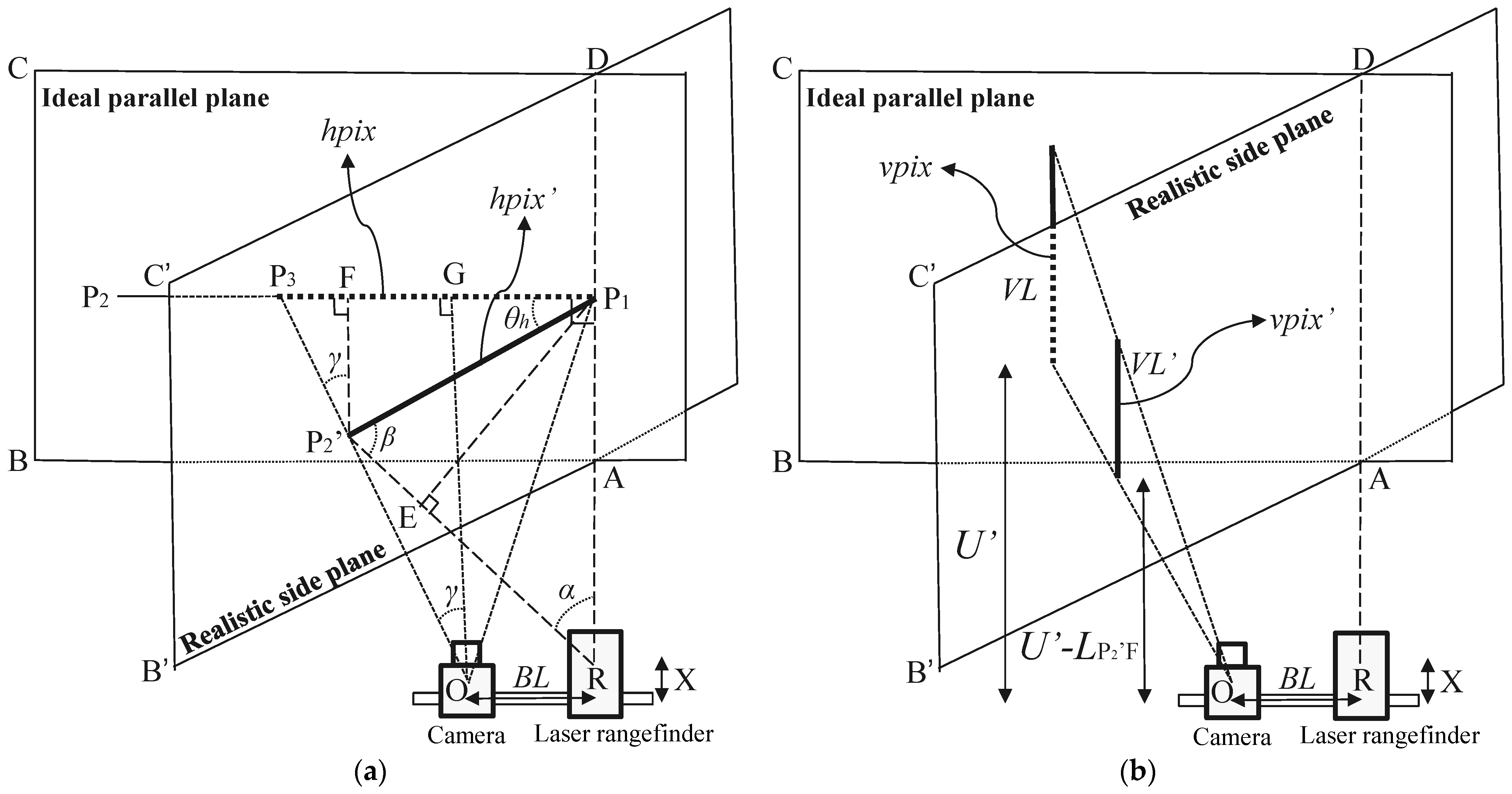
The Gauss camera imaging model calculates the actual physical width L based on the assumption that the object plane is parallel to the image plane. However, it is difficult to achieve true vertical photographing in the practical applications, as shown in Figure 2a, where the appearance of taking photos from the side is exhibited. The pixel distance S in Figure 1 can be divided into λ pixels in the horizontal and vertical directions. According to Equation (4), the real distance L can be directly calculated. However, if the plane rotates around the AD axis, which means the photographing direction is not perpendicular to the target plane, the pixel distance λ would change as ∆λ1 pixels and ∆λ2 pixels in the horizontal and vertical directions, and the calculation method used in Equation (4) would not be satisfied. This deformation in which plane ABCD changes to plane AB’C’D would affect the measurement results.

2.2. Inaccurate Crack Identification Method

Canny edge detection has been considered to be an objective mathematical method [31,32] as the edges are defined as the gradient in the x and y directions generated by the one-order finite difference:
P x [ i , j ] = ( I [ i , j + 1 ] I [ i , j ] + I [ i + 1 , j + 1 ] I [ i + 1 , j ] ) / 2 ,
P y [ i , j ] = ( I [ i , j ] I [ i + 1 , j ] + I [ i , j + 1 ] I [ i + 1 , j + 1 ] ) / 2 ,
where i and j are the locations of each pixel, and I is the pixel value. Then, its gradient amplitude can be computed as
M [ i , j ] = P x [ i , j ] 2 + P y [ i , j ] 2 ,
and the direction as follows:
θ [ i , j ] = arctan ( P y [ i , j ] / P x [ i , j ] ) ,
However, for cracks in reality, redundant edges are always generated and make the results undesirable, and the blurring of crack edges may cause the detected results to be discontinuous. The Canny algorithm calculates the position of the target edge based on the image gradient, which is calculated by referring to the gray values on both sides of the edge, meaning that the places with a large gray difference in the image may be judged as edges. However, the cracks not only have grayscale features but also morphological features. Only using gradient expression will cause many target edges that are not cracks to be identified as crack edges, resulting in noise. Meanwhile, when the gray difference of the crack is small, the Canny algorithm cannot calculate the edge position, as shown in Figure 2b.
Given the irregular shape of the cracks and the interference from background noise, deep learning algorithms are selected by most scholars as the most practical crack detection method. However, for an object as narrow as a crack, each pixel size can affect the accuracy of the results, especially when photographing from a long distance [17,33]. The accuracy of crack segmentation can be analyzed by some indicators, but it still should be refined further during measurement application. Meanwhile, since the proportion of crack pixels in the image is less than the background, this can cause sample imbalance, and the ordinary loss function cannot effectively describe the difference between the predicted value and the ground truth [11,34]. Therefore, combining the advantages of the improved U-net algorithm to automatically extract cracks and the Canny method to accurately calculate the characteristics of crack edges would be a suitable crack measurement approach.

3. Crack Identification and Measurement System

An accurate crack measurement system is proposed in this research. This system is based on the following data: object distance and capturing angle, camera focal length and image processing. The main equipment of the system includes the camera and the laser rangefinder—their optical axes are parallel, and the relative positions are fixed. The rangefinder is used to calculate the position information with the target plane, and the camera is used to obtain the crack images and measure their size. The proposed crack measurement approach is described as follows.

3.1. Measurement System Based on Camera and Laser Rangefinder

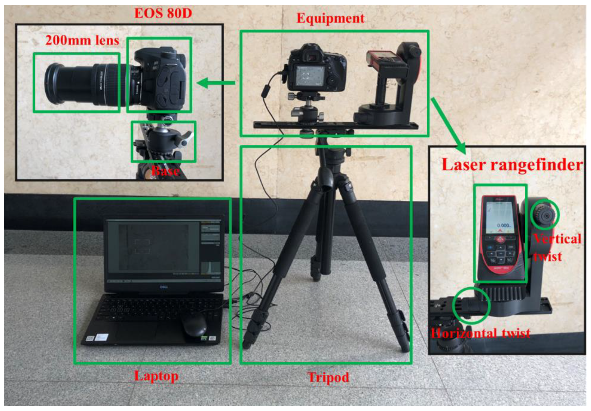
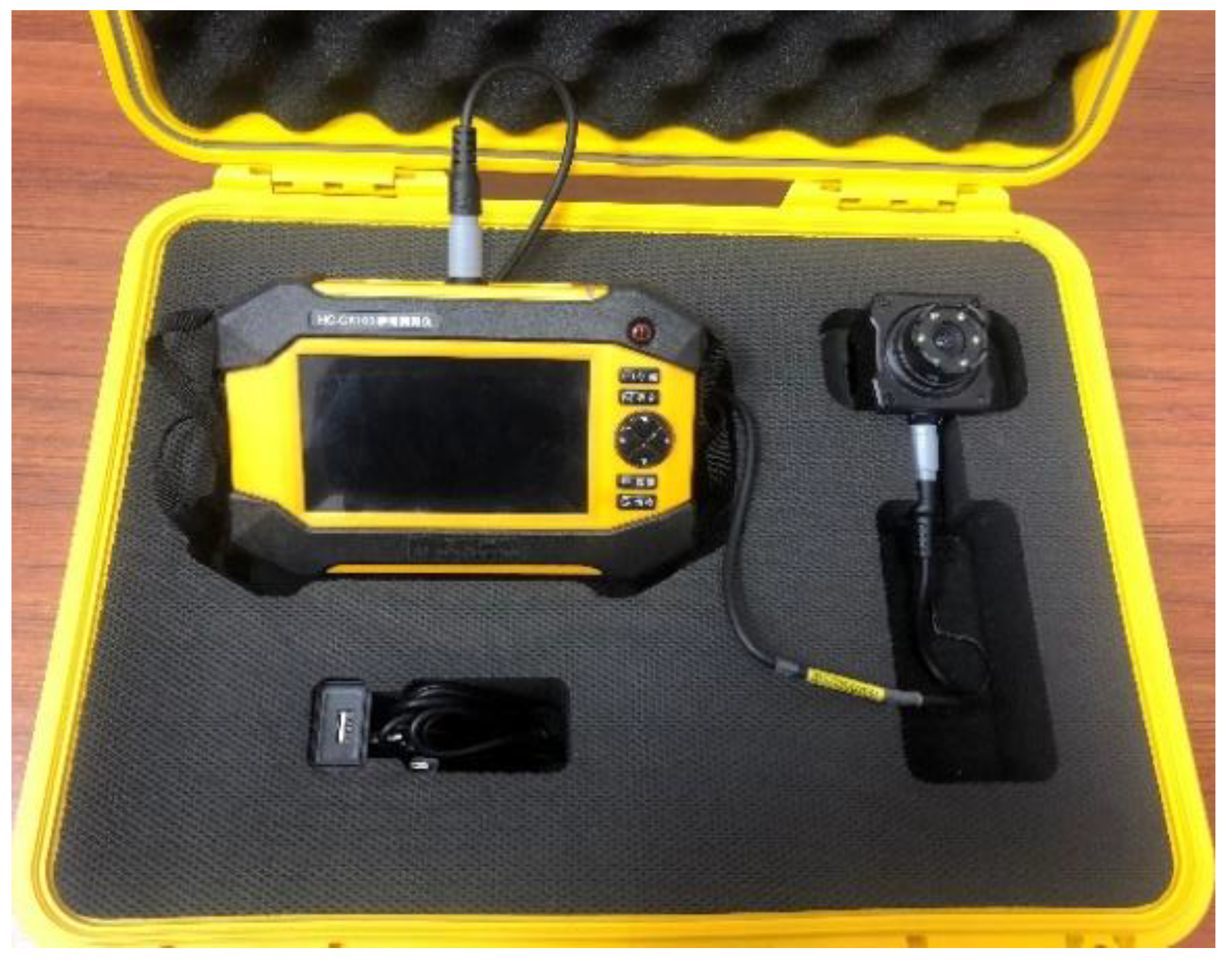
3.1.1. Description of the Proposed Equipment System

The proposed crack measurement system is composed of data acquisition and image processing. As shown in Figure 3, the camera and the laser rangefinder are fixed on bases and are connected by a rod to ensure the optical axis is parallel during use. The equipment is supported by a tripod, which can be placed anywhere. The image acquisition device consists of a Canon EOS 80D camera with EF-S 18–200 mm zoom focal length, and the focal length is fixed at 200 mm to capture target images clearly from a long distance. Another measuring device is the Leica S910 laser rangefinder—in addition to measuring distance, when it rotates horizontally and vertically, the angle of rotation can be recorded. The stability of the distance measured by the laser rangefinder was tested in different environments—after fixing the device, the same point was measured five times, and the measurement distance remained the same, which proved the feasibility of the equipment. The accessory is a base, where two twists can control the horizontal and vertical rotation of the laser rangefinder. A laptop is adopted to store images with a data cable and record the photographing distance and rotation angle information with a Wi-Fi connection.

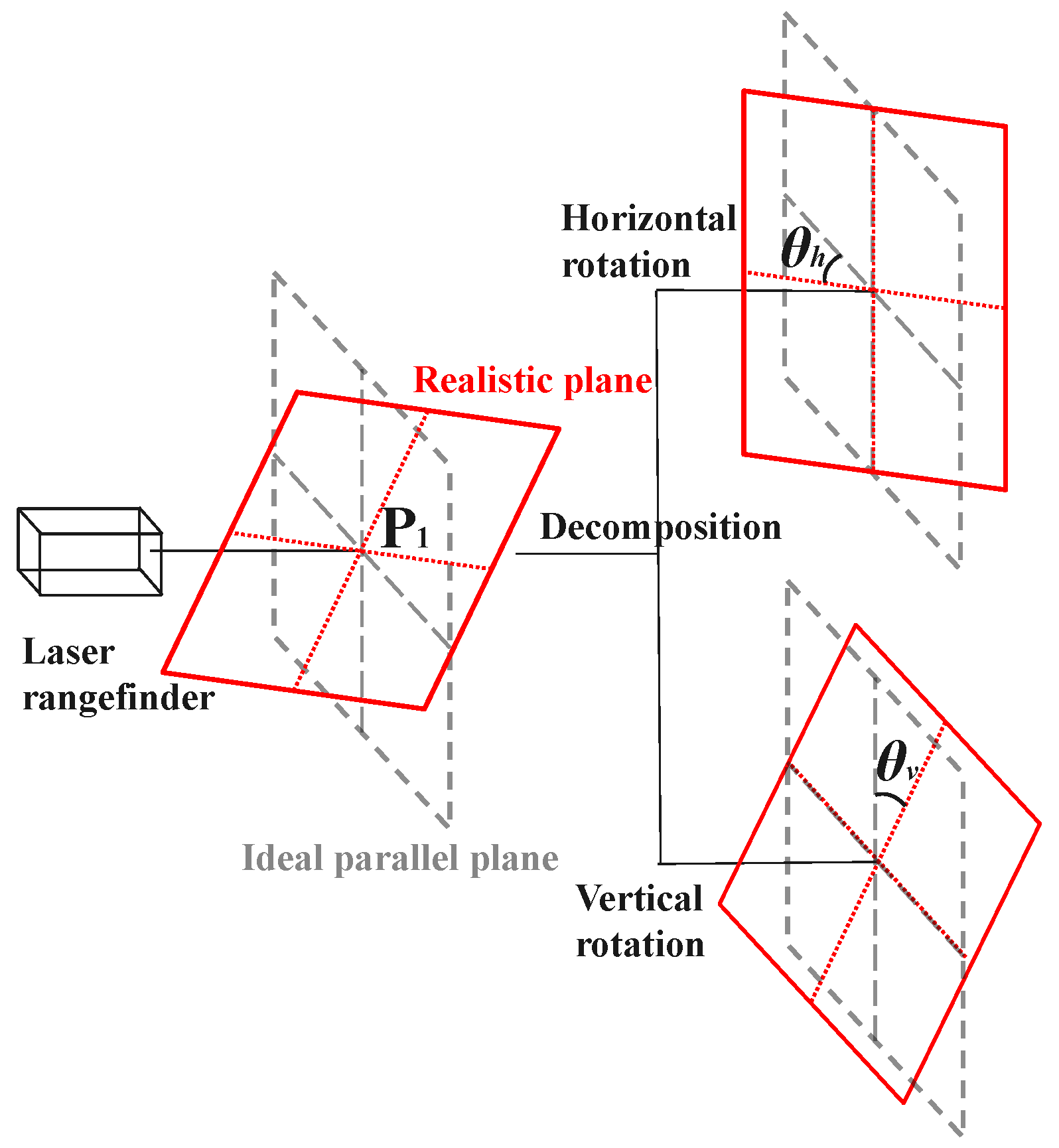
3.1.2. Geometric Transformation Formula of Pixel Length

It can be seen from Equation (4) that the length of a crack can be automatically counted by obtaining the distance to the measured target. However, the distance U obtained by the laser rangefinder is not very accurate, because the camera’s photosensitive sensor and the origin of the laser rangefinder are not certainly in the same plane. This study provides a formula to correct the position of the camera and laser rangefinder as shown in Equation (9):
U = X + U ,
where X is a constant and represents the distance between the camera imaging plane and the origin of the laser rangefinder. Moreover, because of the difference between the half and full frame types, the focal length f involved in the calculation is different from that in the nominal case, and the correction formula is expressed as
f = Y × f ,
where Y is another constant that represents the focal length correction factor. Inputting Equations (9) and (10) into Equation (4), we obtain Equation (11):
L = p i x × ε ( U f ) f = p i x × ε ( U + X Y f ) Y f ,
This formula is a linear transformation in which a relative geometry relationship of equipment is maintained. In practice, if the positions of the camera and laser rangefinder are fixed, the constants X and Y can be uniquely determined.
To apply Formula (11) to the measurement of cracks, if the object plane is not parallel to the images, the main objective is expected to transform the plane to a parallel position on the image plane. The rotation can be decomposed into horizontal and vertical orientation by θh and θv angles, respectively, as shown in Figure 4, and the random measuring point P1 of the laser rangefinder is defined as the center of rotation. Because the rotation is axisymmetric, the side plane generated by horizontal clockwise rotation is taken as an example, and the geometric relation is proposed in Figure 5a. The distance between point P1 and the center point of the laser rangefinder R is the measuring distance U. P2′ is another random point measured by the laser rangefinder by rotating α degrees horizontally on the side plane, and P2 is the same point in the ideal parallel plane. To calculate the horizontal angle θh, the measured distance of the line between points R and P2′ (LRP2) can be decomposed into the sum of LRE and LEP2 and derived as follows:
L RE = U × cos α ,
L EP 2 = L RP 2 L RE ,
L EP 1 = U × sin α ,
β = arctan ( L EP 1 L EP 2 ) ,
θ h = π / 2 β α ,
where the distance U, LRP2 and rotation angle α can be obtained by the laser rangefinder.
If the horizontal imaging pixel length hpix is used to calculate the target length by Equation (11), the result will represent the length LP1P3 instead of the target LP1P2. The pixel length used to calculate the distance can be expressed as
L P 1 P 2 = h p i x × ε ( U f ) f ,
L P 1 P 3 = h p i x × ε ( U f ) f ,
However, since the position of point P2′ is random in the horizontal direction, the proportional relationship between hpix and hpix’ should represent the proportion of the arbitrary horizontal pixel distance on the realistic side plane and the corresponding horizontal pixel distance on the ideal parallel plane. When the camera and laser rangefinder are fixed, the horizontal baseline distance BL can be determined. Since the optical axes are parallel, it can be seen that
L P 1 G = B L ,
L G P 3 = L P 1 P 3 B L ,
γ = arctan ( L GP 3 U ) ,
L P 2 F = L P 1 P 2 × sin θ h ,
L P 3 F = L P 2 F × tan γ ,
L P 1 P 3 + L P 3 F = L P 1 P 2 × cos θ h h p i x = h p i x cos θ h sin θ h × ( p i x × ε ( U f ) U f B L U )
where the relationship between hpix and hpix′ is determined by the rotation angle θh and shooting distance U’. Equation (24) demonstrates that the distance from the center of rotation P1 to a random point in the horizontal direction can be represented by the imaging pixel hpix, and when introducing Formula (24) into Formula (17), the distance LP1P2 can be obtained as follows:
L P 1 P 2 = h p i x × ε ( U f ) × U f 2 U f cos θ h sin θ h × ( h p i x × ε ( U f ) B L × f ) ,
Meanwhile, the horizontal rotation of the target plane will not only create distortion in the horizontal direction but will also cause the displacement and deformation in the vertical direction as presented in Figure 5b and expressed as follows:
V L U + L P 2 F = V L U ,
where VL and VL′ are the vertical length on the ideal parallel plane and realistic side plane, respectively. The vertical length can be calculated by Formulas (11) and (26) with the vertical pixel length vpix, and VL′ is obtained as follows:
V L = V L U × ( U + L P 2 F ) ,
When the realistic plane rotates in the counterclockwise direction, as shown in Figure 6a, the relationship between hpix and hpix′ can be derived similarly. Formula (24) can be converted as follows:
L P 1 P 3 L FP 3 = L P 1 P 2 × cos θ h h p i x = h p i x cos θ h + sin θ h × ( p i x × ε ( U f ) U f B L U )
The length between point P1 and point P2′ in the side plane can be measured by Formulas (17) and (28) as follows:
L P 1 P 2 = h p i x × ε ( U f ) × U f 2 U f cos θ h + sin θ h × ( h p i x × ε ( U f ) B L × f ) ,
Similarly, when the plane is rotated counterclockwise horizontally as shown in Figure 6b, the pixel length in the vertical direction also changes proportionally as presented in Equation (30) as follows:
V L = V L U × ( U L P 2 F ) ,
It is worth noting that the proposed system is based on the camera located on the left side of the laser rangefinder, and the base line distance BL does not only exist in the horizontal but also in the vertical direction. However, it can be seen from Formulas (24) and (28) that when the camera is close to the laser rangefinder or measured from long-distance, the shooting distance U′ is much larger than the base line distance BL, implying that BL can be ignored to simplify the model.
The position of a laser point is a key parameter in the proposed system that represents the center of target plane rotation and the origin of calculating the distance between pixels on both sides of the crack. As a laser point is usually a red circle or ellipse, as shown in Figure 7a, the center is identified using a circular Hough transform, which is widely adopted in much image processing research due to its sub-pixel accuracy and high stability [35,36]. Since the color of the laser point selected in this study is red, among the multiple circles identified in the circular Hough transform, the reddest one is considered to be the laser point as shown in Figure 7b, and the location in the images is recorded.
The proposed measurement model is composed of a laser rangefinder and a camera with a fixed relative position and parallel optical axis. To calculate the target length by the captured image pixel, the target plane is decomposed into horizontal and vertical rotations, and the center of rotation is the direct measuring point by the laser rangefinder. Rotation angles can be calculated from another point measured by the laser rangefinder, which can be used to derive the pixel length conversion formula, and the positional relationship from a random point on the image to the center of rotation can be determined. Therefore, the distance between two random points on the image, such as the edge of a crack, can be obtained by the distances and angles measured by the laser rangefinder.

3.2. Crack Segmentation Based on U-Net Algorithm

Image processing is an essential procedure for long-distance measurement based on computer vision. The areas of cracks will be obtained by the U-net algorithm; then, the edges are refined by the Canny algorithm; and finally, skeleton extraction algorithms will generate a crack skeleton to calculate the crack width by pruning based on the partition of the boundaries [37]. Crack area extraction based on U-net is the most important step and is described below.

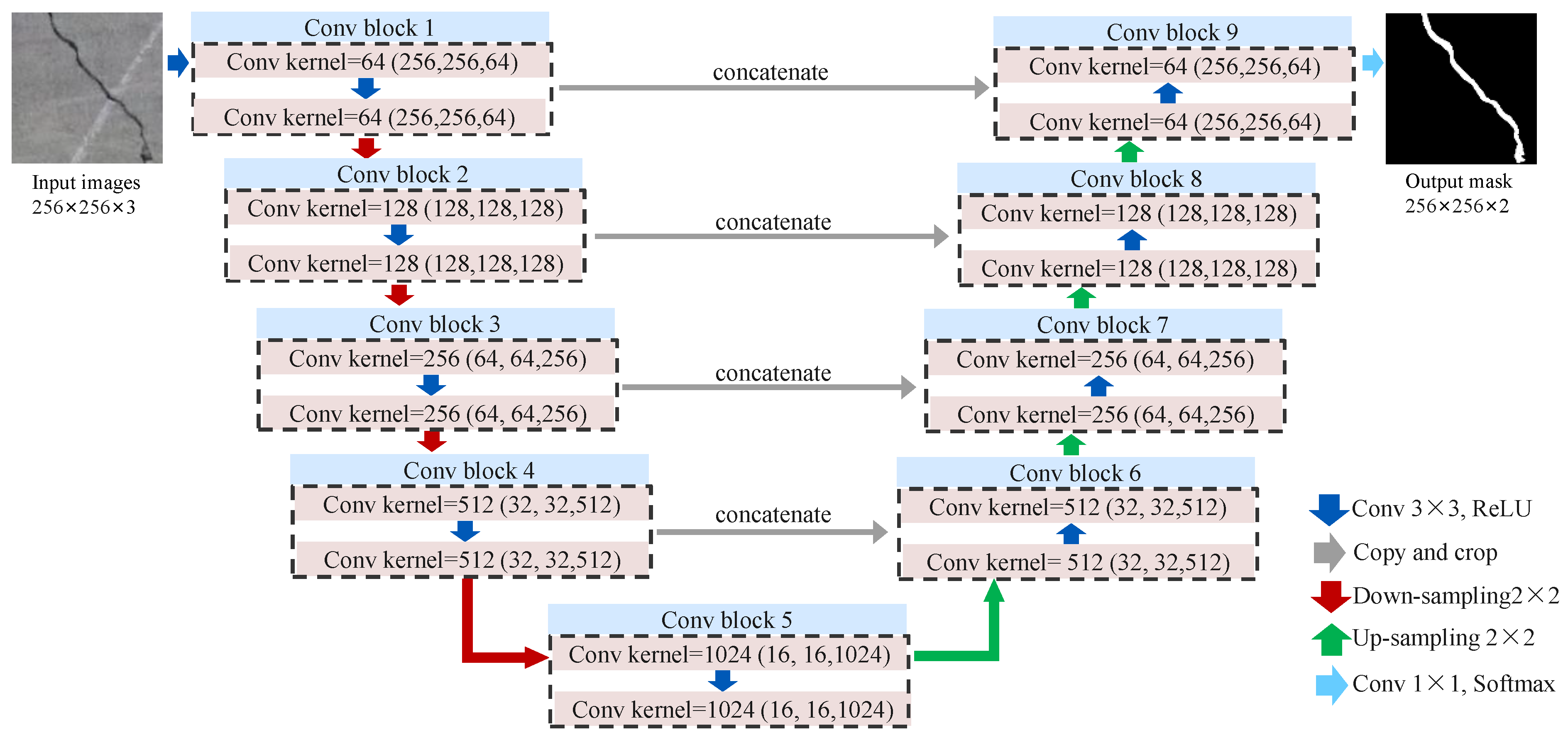
3.2.1. Architecture of U-Net

The architecture of U-net including inputs, outputs and intermediate layers is as shown in Figure 8 [14,15,16]. The left part is the contracting path, and the right part is the expansive path. As the input 256 × 256 size images pass through the contracting path, high-resolution features are extracted by several convolution filters (Conv) with 3 × 3 kernels to compress the images into a multi-channel feature map. The aims of proposing the activation function behind Conv are to add nonlinearity to the neural network to fit more nonlinear functions. The ReLU activation function is a commonly used activation function to strengthen nonlinear properties and is defined as follows:
ReLU ( x ) = max ( 0 ,   x ) ,
In order to reduce the number of parameters in the network and the risk of overfitting, a down-sampling operation is selected as an intermediate process of connecting each Conv block in the contracting path. The max-pooling operation, which is one of the methods of down-sampling, has been widely adopted and has been proven to preserve the features well. After encoding procedures, the features are delivered to the expansive path. Contrary to the left part of the architecture, the expansive path gradually upsizes the computed data shape to the original input image size to precisely restore and locate features. Simultaneously, the paralleled features map from the contracting path is directly passed to the expansive path by concatenation. In the end, the final Conv layer is designed with a size of 1 × 1 to transform the output images into binary at the same size, storing each classification into each pixel. To compress the classification results in a normalized form, the Softmax function is selected for normalization as follows:
S o f t m a x ( y j ) = e Z j i = 1 N e Z i ,
where N is the total number of categories, j is the pending category, and Z is the delivered weight from the previous Conv layer.

3.2.2. Loss Function

The loss function is a main indicator describing the deviation between the predicted results generated from the network and the ground truth. The target of training the model is to minimize the loss value to make the final segmentation more accurate. In previous studies of crack semantic segmentation, several classic loss functions including cross-entropy loss function, dice loss function [27], focal loss function [10] and some combinations [14,17] have been widely adopted. Furthermore, data imbalance is a problem that exists in crack segmentation tasks; since the crack pixels occupy a small proportion of the total, this may cause a training weight offset.
In order to obtain the accuracy loss values during the training produce and solve problems caused by the data imbalance, a combination of generalized dice loss (GDL) and cross-entropy loss (CE) is selected as the loss function. The GDL function can solve crack segmentation as the weight of each level is inversely proportional to class frequencies [11,34,38] and can be expressed as
L GLD = 1   2 l = 1 2 w l n r l n p l n l = 1 2 w l n r l n + p l n ,
where rln represents the ground truth of class l at n pixel position, pln is the corresponding predicted value generated by the model, and wl is the weight of each class, expressed as
w l = 1 i = 1 N r l n 2 ,
where N is the number of training samples. The CE function is expressed as [39]
L CE = n = 1 N r n log   p n ( 1 r n ) log   ( 1 p n ) ,
The loss function of U-net in the training process is given by
L = L GLD + L CE ,
Applying the combination of GLD and CE can solve the problem of the excessive background ratio in order to better extract the cracks.

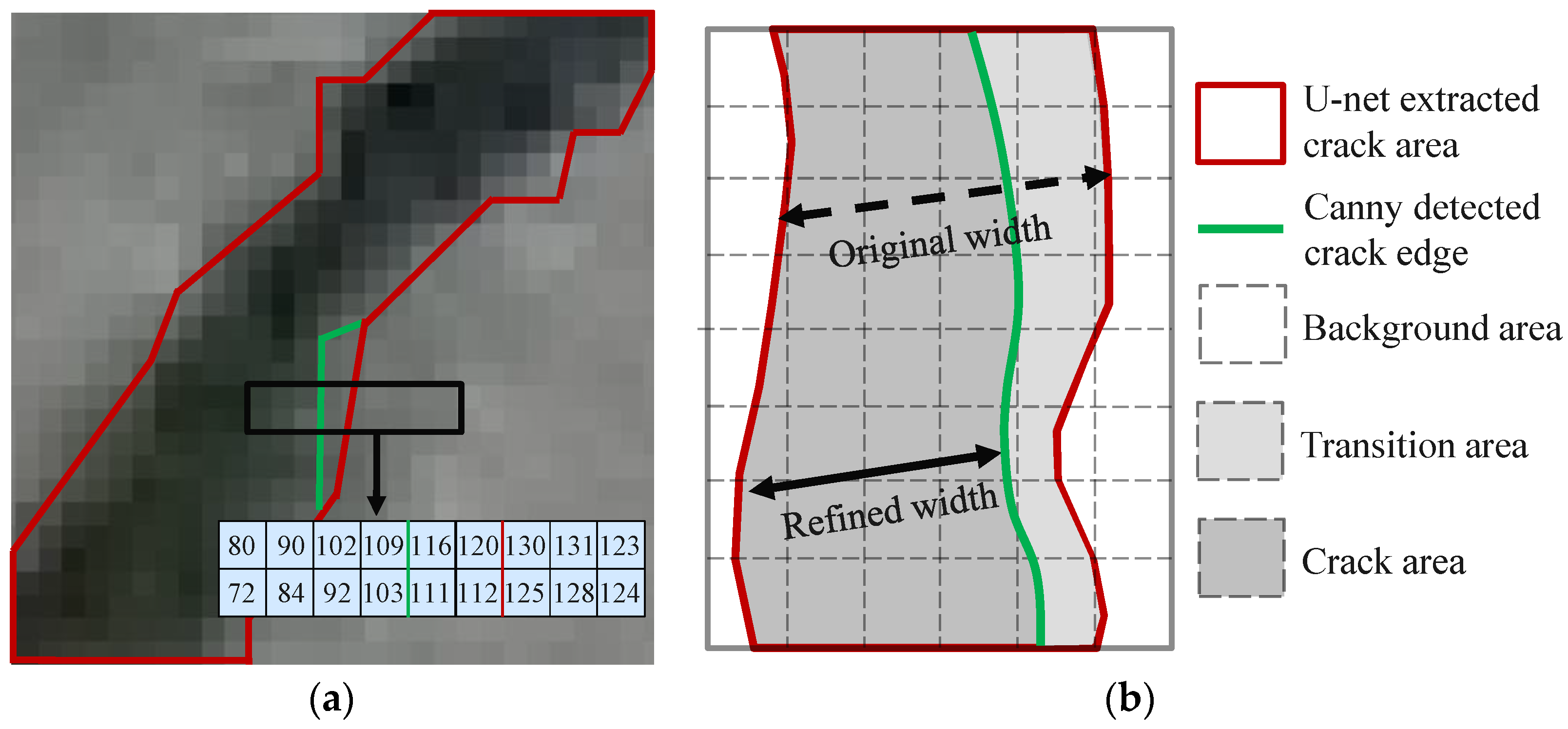
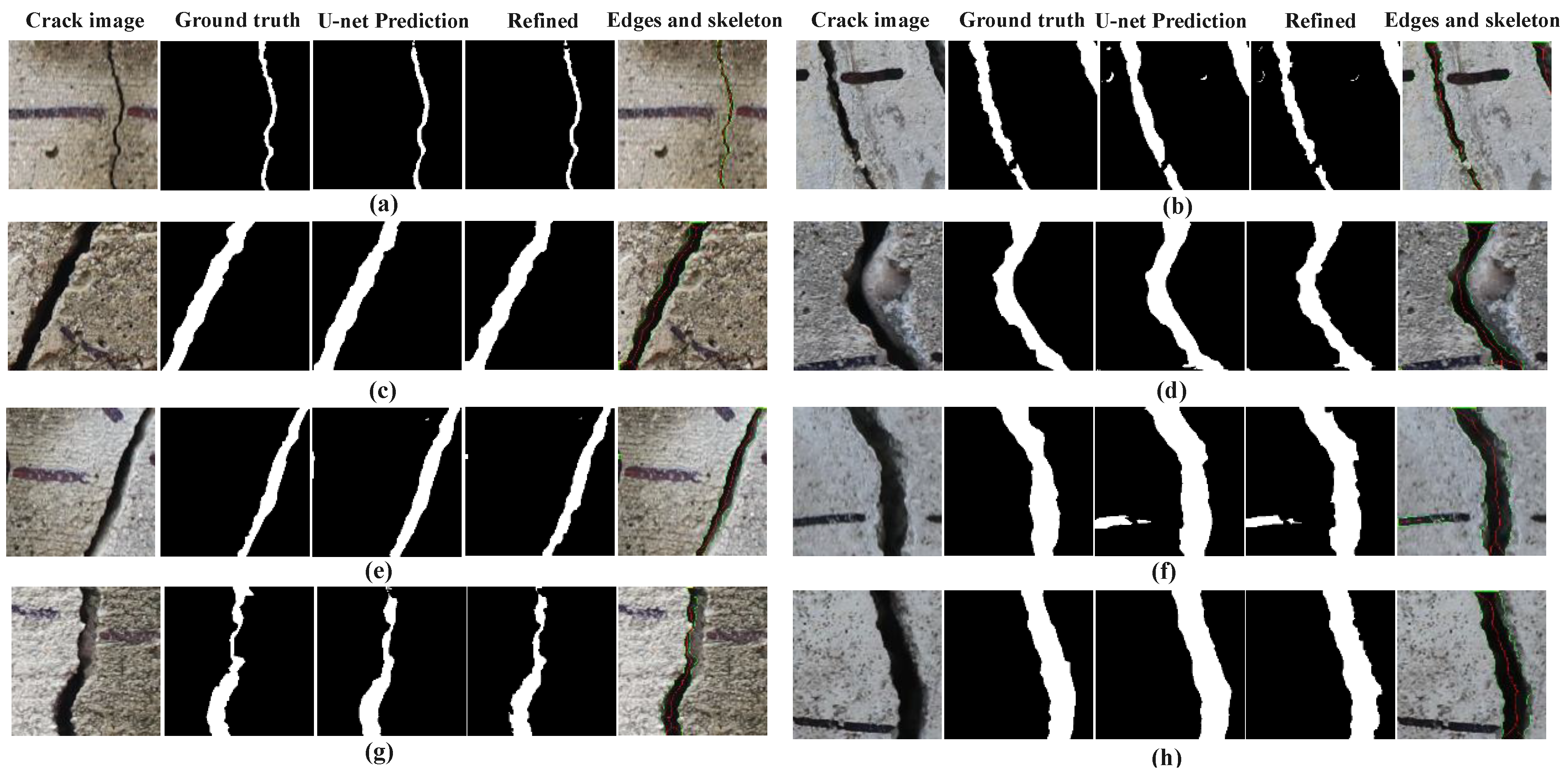
3.2.3. Edges Refined by Canny Algorithm

After processing with the U-net algorithm, the areas of cracks in each image can be identified and extracted. Nevertheless, due to the imperfection of the model or inaccurate datasets for training, the edges of cracks generated by the U-net algorithm are a little different from the results generated by the Canny algorithm. As shown in Figure 9a, the boundary between the background and the crack is usually not very distinct, and there will be a transition area of a gray gradient that is a few pixels wide, which usually results in misjudgment of the crack boundary. Therefore, the crack edges need to be refined using the Canny algorithm. If the U-net segmented crack areas include Canny detected edges, the edges of the crack will be refined to the Canny results. Because the gradient of the gray image is not uniform, the edges generated by the Canny method are often discontinuous. In this case, both ends of the edge are extended in the normal direction, and the intersection with the original boundary will be replaced, as shown in Figure 9b. In this way, the edges of the cracks can follow specific mathematical standards and provide a basis for verifying the width of the cracks.

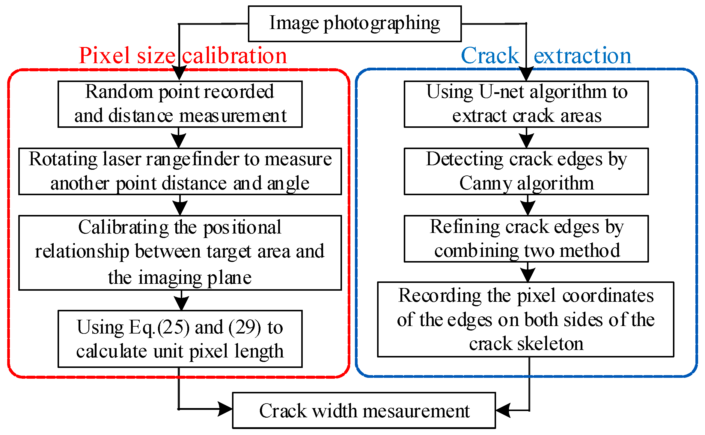
3.3. Process of Crack Measurement

The distance and angle of the target plane are measured by the laser rangefinder, and the crack image captured by the camera is segmented by the U-net algorithm. The automated measurement process is currently limited because the unpredictable environment has a greater impact on crack extraction. In this study, we proposes a semi-automatic algorithm for crack measurement; the main steps of the pixel size calculation and crack extraction algorithm are summarized in the flowchart in Figure 10 and described in detail as follows.
Step 1: Center point determination. A random point measured by the laser rangefinder is considered as the center point of the target plane, and the position of the center point in the image is recorded by the camera.
Step 2: Horizontal and vertical rotation angle measurement. The horizontal angle and distance can be calculated by rotating the laser rangefinder horizontally, and the same procedure can be applied to acquire the vertical angle.
Step 3: Pixel length translation. The distance between a random point and the center point on the image can be calculated according to Formulas (25) and (29), and the pixel length can be translated to the actual distance.
Step 4: Crack segmentation. After calculating the pixel length, the areas of the cracks in the captured images are segmented by the improved U-net algorithm, and the model is trained previously based on several concrete images taken in different conditions.
Step 5: Edges refined. The crack images are processed by the Canny algorithm again, and if the generated edges are in the crack area segmented by U-net, the crack will be refined.
Step 6: Crack width calculation. After obtaining the refined crack, we extract the skeleton and the pixel width of the crack perpendicular to the direction of the skeleton and finally calculate its actual width.
To evaluate the quality of the trained model, four commonly adopted indicators for neural network evaluation are referenced, which are precision, recall, F1-score and IoU, respectively, defined as
P r e c i s i o n = T P T P + F P ,
R e c a l l = T P T P + F N ,
F 1 = 2 p r e c i s i o n × r e c a l l p r e c i s i o n + r e c a l l ,
I o U = T P T P + F P + F N ,
where TP is true positive, representing the number of true positive pixels; FP is false positive, representing the number of false positive pixels; and FN is false negative, representing the number of false negative pixels.
Data acquired from the object plane are adopted to extract the crack width. Different measuring objects are evaluated by several performance criteria, such as the mean absolute error (AEmean), the root mean squared error (RMSE) and the coefficient of determination (R2), which are shown as follows.
A E mean = 1 N i = 1 N | L M ( i ) L ¯ ( i ) | ,
R M S E = 1 N i = 1 N ( L M ( i ) L ¯ ( i ) ) 2 ,
R 2 = [ i = 1 N ( L M ( i ) L ¯ M ) ( L ( i ) L ¯ ) ] 2 i = 1 N ( L M ( i ) L ¯ M ) 2 i = 1 N ( L ( i ) L ¯ ) 2 ,
where LM and L ¯ M represent the measured and the average measured values, L and L ¯ denote the standard and average standard values, and N is the number of objects. The optimal results should be verified with the minimum mean absolute error, root mean squared error and coefficient of determination close to 1.

4. Case Study

The proposed procedure is verified by using the combination of the camera and laser rangefinder shown in Figure 3 to measure real crack width. The standard size of the crack is measured by the HICHANCE-CK103 crack width measuring instrument as shown in Figure 11. To verify the accuracy of the adopted instrument, a crack scale board is adopted as shown in Figure 12a, and six groups of the standard widths are measured, including 0.08 mm, 0.2 mm, 0.5 mm, 1 mm, 1.5 mm and 2 mm, respectively [40]. The measurement results are stable, and the errors are kept within 0.01 mm, as shown in Figure 12b, which proves that the instrument can be used for crack width measurement. The training process of U-net was performed on a workstation with a single GPU device (NVIDIA Quadro P5000) and CPU (Intel i7 8700K). The environment of the training code is Python 3.8, and the software MATLAB R2018a is used to program the measurement procedure.

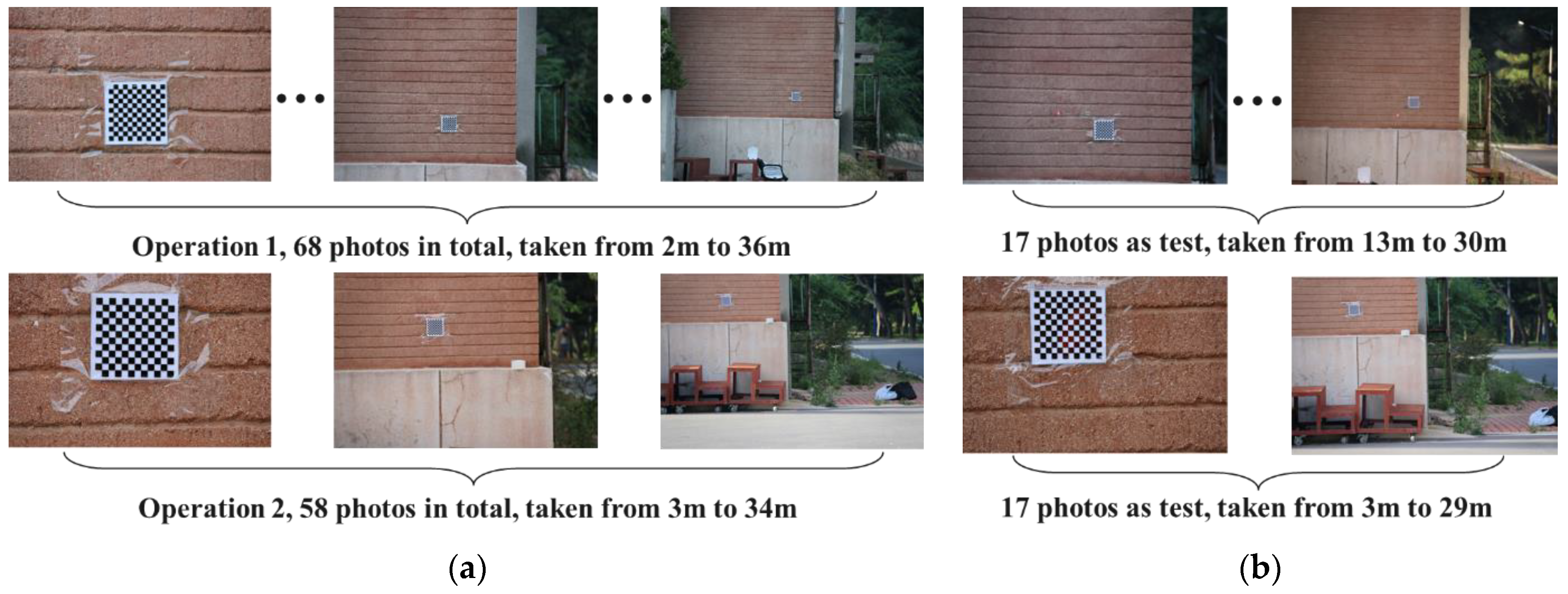
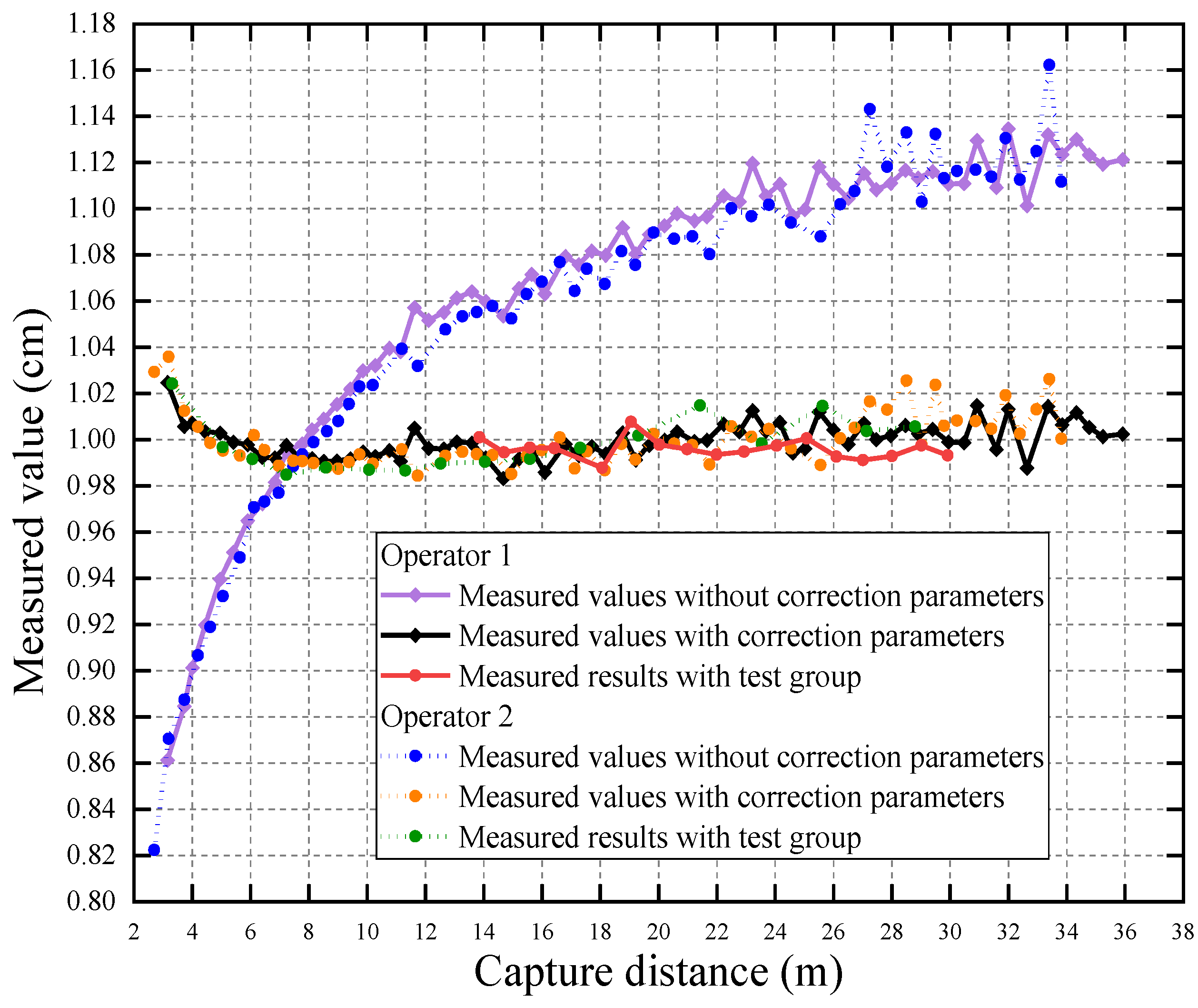
4.1. Determination of System Parameters

The first step consists of determining the parameters of the system in Equation (11), which are uniquely determined when the system is fixed. A calibration board is fixed on the wall as shown in Figure 13—each grid size L is a standard of 1 cm, and the average length of all grids of the calibration board is set as the target. the measuring system in Figure 3 is used to capture the calibration board vertically from 2 to 36 m, and the distance from the system to the calibration board by laser rangefinder is recorded. In order to check the variability of the distances measured by the laser rangefinder, two sets of data are obtained by two operators separately. The basic parameters f is 0.2 m, and U is the measured value; the unit pixel size is 4.4 × 10⁻⁶ m, and the unit pixel aspect ratio is set as 1 as expressed in the camera manual. The parameters X and Y are calculated as 1.1306 and 1.1421 by the least squares method, respectively. Another 34 images of the calibration board are measured as two test groups, and the results are presented in Figure 14. It can be seen that after correcting the parameters, the measurement results are concentrated near the true value. However, some fluctuations occur in the measurement range more than 30 m, which could be due to the instability of the laser rangefinder or the unclear images. Therefore, further measurements were taken within 30 m. A comparison of the measured values corrected by system parameters is shown in Table 1AEmean changes from 0.0538 to 0.0074 cm after correcting coefficients, also greatly improving in the test group; this trend is also reflected in the criteria RMSE. Meanwhile, these experiments prove that the unit pixel size and unit pixel aspect ratio conform to the contents of the camera manual. The object length measured by the system with correction parameters is more accurate, and better fitting results than those using Equation (4) can be obtained.
Note that the system parameter tests were confirmed before practical application, and the camera parameters (such as focal length) and measurement setup can be adjusted for different circumstances. Because the base line distance BL is about 20 cm and much less than the measured distance U, as stated in Section 3.1.2, the value of BL is ignored in the following experiment.

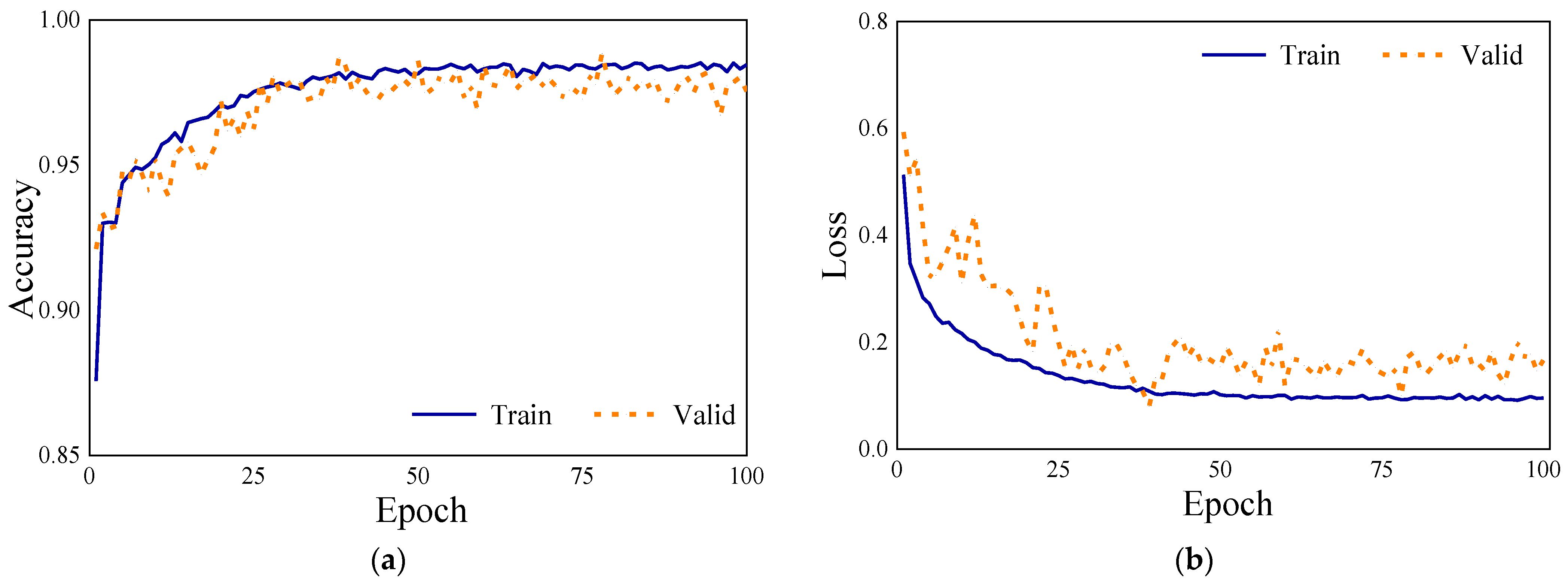
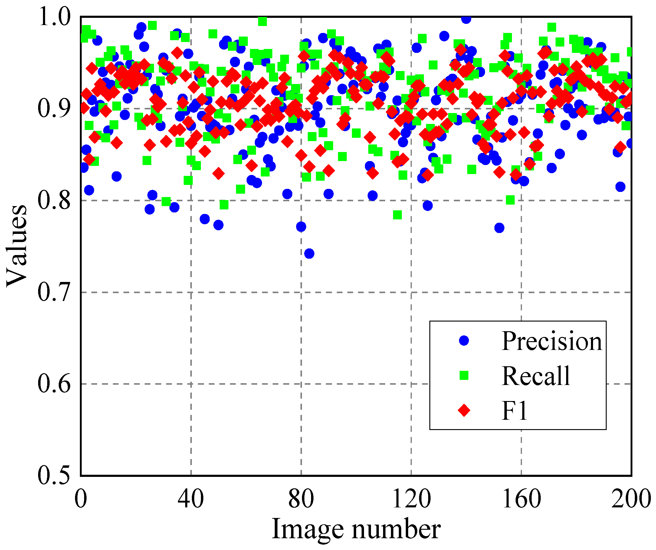
4.2. U-Net Model for Concrete Crack Segmentation

For the training process, a total of 1800 images with the resolution of 256 × 256 are taken as the training dataset, and 500 images are set as validation. These images are taken from several concrete walls at different distances, angles and environments for the generality of the model.
Figure 15 illustrates the accuracy and loss over epochs, and a good convergence of the neural network is indicated. The accuracy is the ratio of correctly predicted pixels to the total pixels, and the loss values are calculated by the loss function in Equation (36). The accuracy rate of model reaches 0.98 during training, while validation is slightly lower. Figure 15b shows the decrease of the loss value in each epoch. To further evaluate the performance of the U-net model in crack segmentation, the model is tested with the testing dataset. The test dataset contains 200 images, which are not used in the training and verification process. Precision, recall and F1 values of each image in the test dataset are shown in Figure 16, and the average values of three indicators in training, validation and testing datasets are presented in Table 2. The result is similar to the values from Zhang [17], and the accuracy of segmentation during each procedure is more than 90%, which indicates the good performance of the model and low overfitting of results.

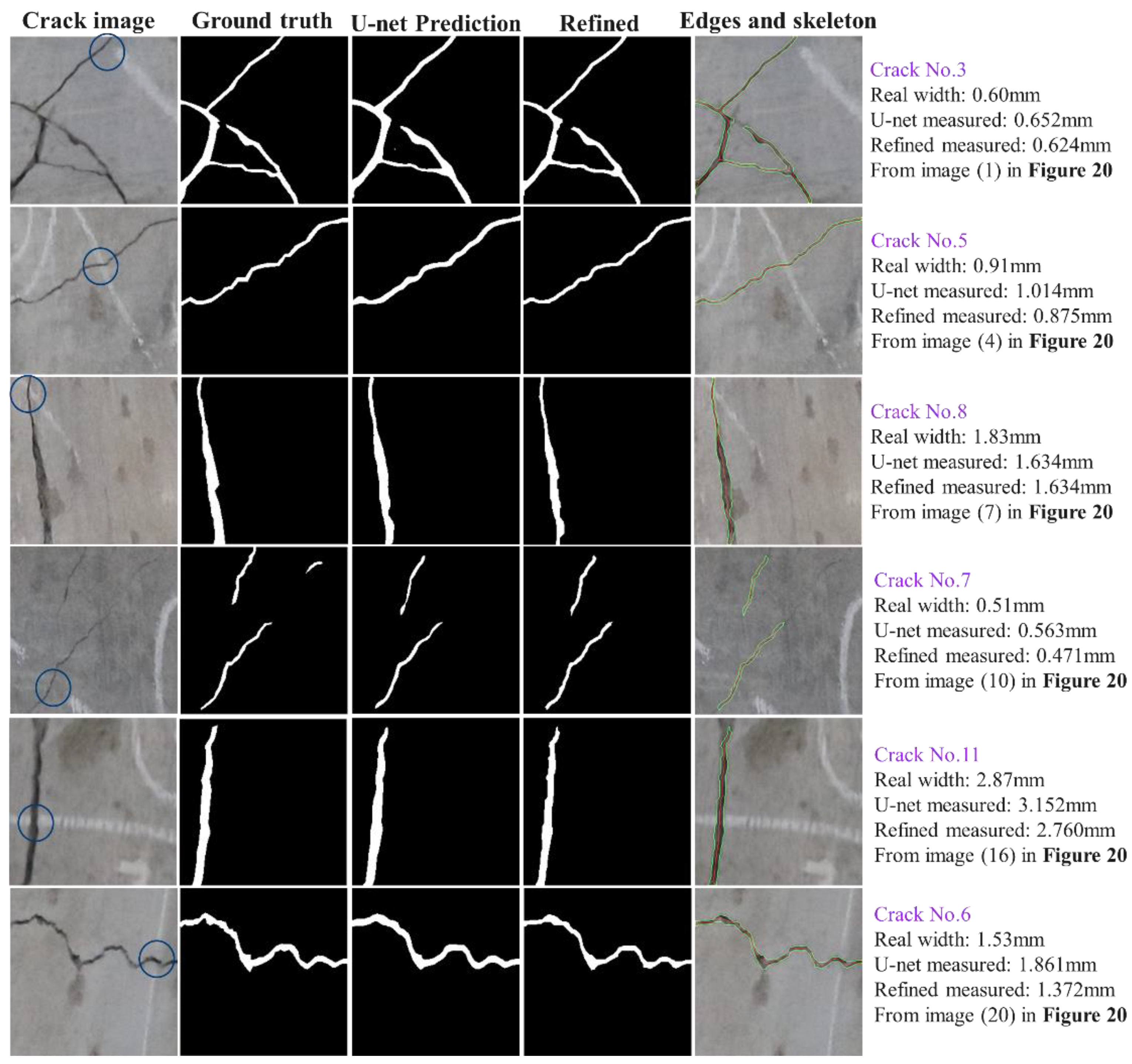
4.3. Crack Measurement Tests in Lab

To comprehensively evaluate the errors of the system and analyze the influence of errors caused by equipment, algorithms and environmental factors, several experiments are carried out step by step. The accuracy verification of the proposed system is mainly divided into the following steps: firstly, the proposed combination of the camera and laser rangefinder is used to measure the size of the grid on the calibration board from different distances to evaluate the systematic error; secondly, standard cracks are artificially generated and segmented by the proposed combination of the improved U-net segmentation algorithm and Canny method to analyze the practicality of the algorithm; finally, the system is applied to the actual cracks on the concrete wall in the laboratory, outfield and concrete dam.
The calibration board Is the same as presented previously with a 1 cm grid size and is measured from 9 m to 30 m. Some measurement scenarios are shown in Figure 17, and the results are presented in Table 3. Since there are many grids on the calibration board, the average value of the measurements is used for comparison. The maximum error occurs at the position with the largest horizontal angle, which is −0.216 mm, and other large errors also occur at larger distances or angles. Meanwhile, it can be seen that the influence of angle on the measurement results is greater than that of distance. The reason for this tendency is that a larger measuring distance or bias angle will reduce the number of pixels that the target occupies in the image, resulting in a larger effect of image resolution and unit pixel size on the target size. Since the corner point extraction algorithm of the calibration board is relatively mature and accurate, the experimental error basically represents the systematic error of the measurement equipment.
Moreover, five artificial cracks with standard width of 7.2 mm, 4.2 mm, 2.3 mm, 1.25 mm and 0.7 mm are placed on the plane as shown in Figure 18, and the widths are measured by the crack width measuring instrument. Each crack is measured three times, and the average values are used for analysis; the results are presented in Table 4. Similar to the aforementioned systematic error analysis experiments, larger errors also occur at positions with larger capturing angles, and the errors are minimal when photographed vertically. The average error in each position is 0.066 mm, 0.079 mm, 0.046 mm, 0.078 mm and 0.072 mm, respectively, and the maximum error does not exceed 0.2 mm, which satisfies the accuracy requirements of practical application.
To verify the accuracy of the image-measured methods proposed in this study and the effect of capturing angle and distance on measurement results, 12 natural cracks on a concrete wall are selected as a test sample, as shown in Figure 19. As the standard widths of the cracks are measured by an instrument, as shown in Figure 11, 20 images of the concrete wall acquired in different positions have been chosen to compare the widths with standard values; the specific photographing distances and angles are shown in Figure 20. Due to the size of the experimental site, the captured distances L and horizontal angle θh change from 5 to 20 m and −65° to 50°, and there is a red laser point on each image, representing the set measurement center points.
After measuring the distance and rotation of the object plane, some sample crack segmentation and measurement results on each procedure are shown in Figure 21. It can be observed that the crack pixels can be extracted by the U-net model, and the refined method by Canny algorithm can improve the crack width measurement accuracy. Of these, crack no. 8 is not refined due to the good performance of U-net segmentation. The larger error values occur in images 7 and 20, which are captured at larger horizontal angles. As the larger photographing distance and angle cause the unit pixel size ε to be larger, the errors caused by other parameters in Formulas (25) and (29) would be magnified, and larger errors in measurement may result. To confirm the measurement accuracy of the proposed system, the results of the width of each crack in each image are shown in Figure 22. Except for the areas not captured in the images, most of the cracks were detected and gave accurate results. Crack no. 1 and crack no. 7 are not detected in some images, because the narrow crack width resulted in a small number of captured pixels; for instance, the width of crack no. 1 only contains 1 pixel during photographing at a larger side angle, and the shallow depth of field of the camera causes a blur at the edge of the target plane, which makes the narrow crack unrecognizable.
The comprehensive evaluation index of each crack is presented in Table 5, in which the width value of undetected cracks is calculated as 0. The AEmean and RMSE of most cracks are less than 0.1, which indicate the robustness of the measurement system to different crack widths. The large errors occur in cracks nos. 1 and 7; since the crack is too narrow and the camera resolution is not sufficient, the unit pixel length is larger than the crack width. Except for undetected cracks, Table 6 illustrates the impact of different photographing angles and distances on the measurement results. The measurement result of the proposed measurement system is accurate in most positions, and the average absolute error is less than 0.2 mm. The minimum R2 occurs in image 6, image 7, image 19 and image 20, which are at a more than 50° horizontal angle to the target plane, and the greatest influence on the results is the undetected cracks in the image. Meanwhile, better measurement results appear in image 1 and image 12, because they have less distance and angle to the target plane, resulting in a larger number of pixels occupied by cracks. The test results prove that the measurement system proposed in this study can measure concrete cracks from any angle and distance—the maximum error is less than 0.3 mm and can be reduced to 0.15 mm when photographing closer. Similar to the previous artificial standard cracks, the capturing angle is the factor that has the greatest impact on the measurement accuracy. Tests in a laboratory show that the capturing angle should not be greater than 50° and the measurement distance should not be larger than 30 m for the equipment under this study.

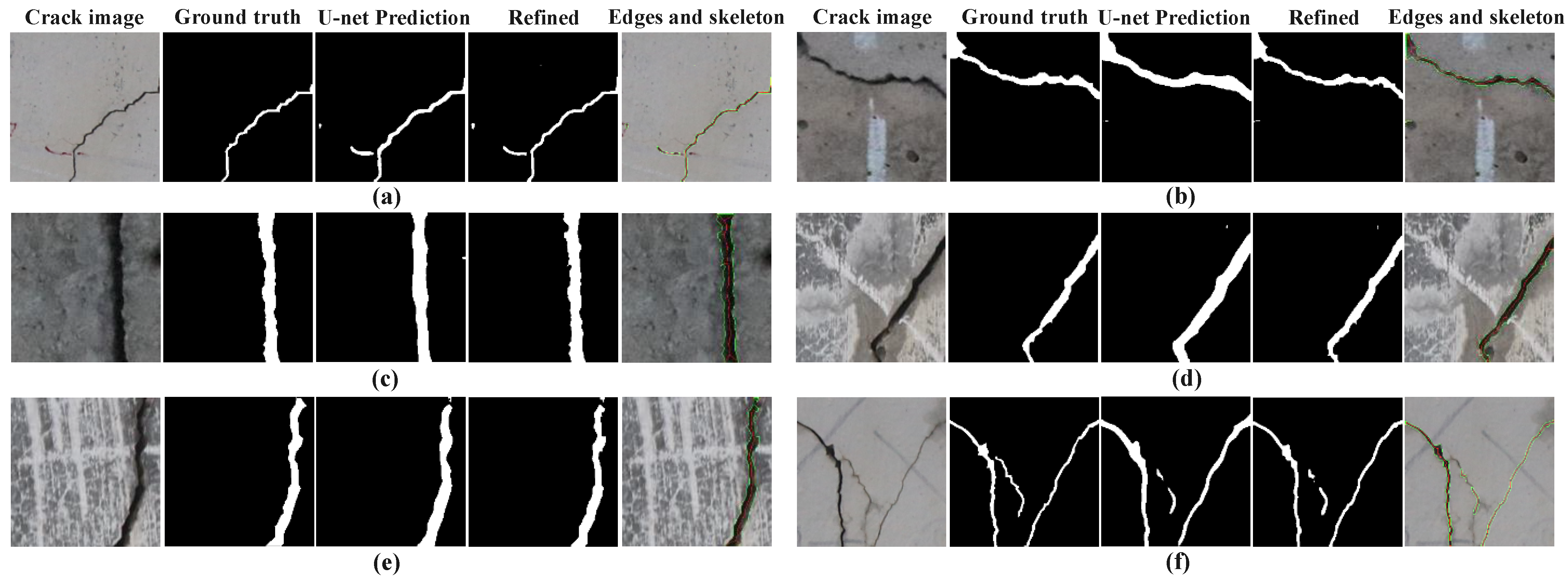
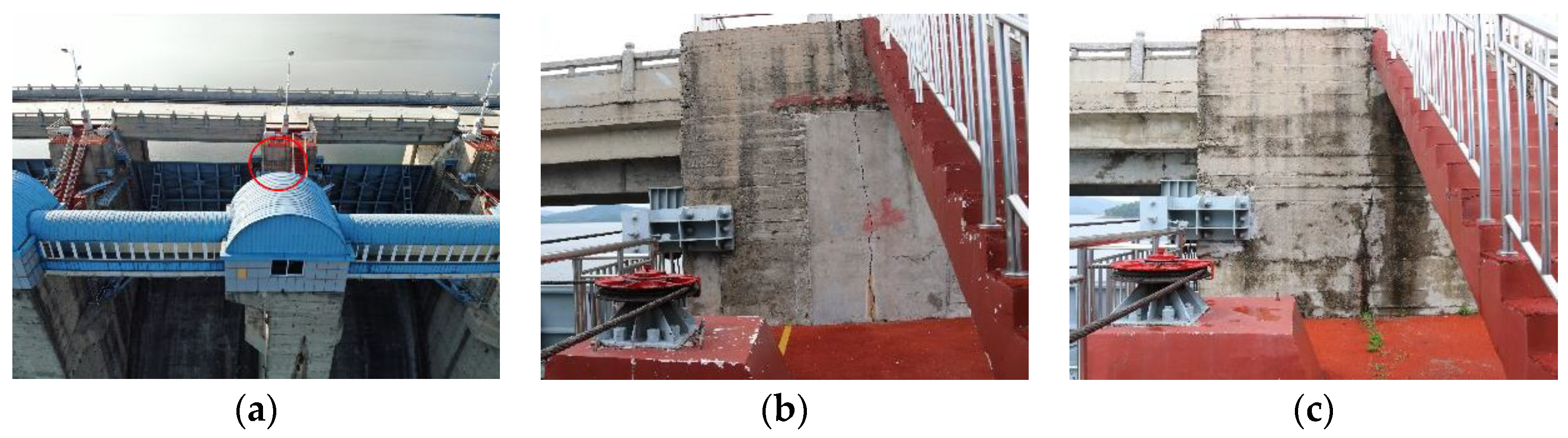
4.4. Concrete Crack Detection Using the Proposed System

The practicability of the proposed system was verified by performing crack width measurement on several concrete walls, and the trained model for crack segmentation is the same as the previous model. Compared with the ground truth, the crack area can be extracted from different backgrounds as shown in Figure 23b,d. In addition to the artificial marks wrongly identified as cracks in Figure 23a, blurred boundaries can affect the effect of crack segmentation as Figure 23c. When the background and the cracks are more distinguished, as in Figure 23e,f, the cracks can be better extracted, but the unclear crack in (f) is not completely identified. The boundaries of cracks on concrete structures are usually not clear enough, which cases the edges of U-net segmentation results to be different from the results of the mathematical calculation, and the refinement operation significantly improves the effect of crack extraction. The measurement procedures were carried out under different photographing distances and angles—details are shown in Table 7. The trend of error distribution is similar to the previous verification results, and the maximum error occurs at the furthest position, which is calculated as −0.15 mm measured from 15.647 m. For cracks with a small captured angle, the relative error is less than 5%.
The proposed system is also applied to a concrete dam to measure the cracks on the concrete pier, as shown in Figure 24. To facilitate verification, the capturing distance and angle are small. Cracks on a concrete dam are usually composed of complex backgrounds, making the segmentation effect different. To analyze the algorithm’s ability to extract cracks, the captured images are divided into sizes of 256 × 256, and some typical examples are used for analysis as shown in Figure 25. The artificial marks are still misidentified as cracks in Figure 25b,f. The partial recognition effect of crack form changes is affected by the blurry boundaries, as in Figure 25d,g. Furthermore, Figure 26 presents some original captured crack images and the combination of each 256 × 256 size image after crack segmentation and Canny processing. With the simple background as shown in Figure 26a,c,e, the crack extraction results are consistent with the actual case, and the misidentified noise and artificial marks are reduced. However, when the concrete surface is uneven or full of holes, as in Figure 26b,d,f, the darker part of the image will be mistaken for a crack.
The measurement results of the cracks on the pier of the concrete dam are presented in Table 8. Except for two cracks that are undetected, the relative errors are less than 5%, which conforms to the trend of the accurate measurement of large cracks captured at close range. Due to the crack protrusions, the specific error is larger than in the lab, and some errors are more than 0.2 mm. Comparing the crack measurement results in another study [25], the absolute error in this system is a bit larger due to the longer distance and wider width, but the relative errors are similar—most are less than 5% and can satisfy practical application.
The mathematical model of the proposed camera and laser rangefinder can efficiently measure the unit pixel size, and the improved U-net segmentation algorithm can properly extract cracks. It can be demonstrated that the proposed approach for crack width measurement is verified to be efficient and accurate.

5. Discussion

This paper proposes a novel system combining a camera and laser rangefinder for non-contact measurements from a long distance and adopts the combination of the improved U-net segmentation algorithm and Canny edge detection method to accurately measure the crack width of the concrete structure. This approach is very effective for solving crack measurement problems under non-contact conditions.
Compared with traditional vertical photographing methods or other non-contact computer vision measurement research using a laser rangefinder [41], the proposed system considers the influence of pixel distortion caused by non-vertical photographing and calculates the unit pixel length of the image captured at any angle. Similar to the previous research, the photographing distance is measured by a laser rangefinder, but the error is corrected by parameters to make the results more accurate. This system adopts computer vision but without large machines [42], making it convenient for practical application. Moreover, in terms of the crack extraction algorithm, the method proposed in this paper also makes improvements. For the problem of data imbalance caused by the low crack pixel proportion in the image, an improved U-net algorithm is proposed by referring to the previous research and achieves good performance in the dataset [11,17]. In addition, the Canny algorithm is introduced to refine the extracted crack edge to improve the measurement accuracy. Regarding the measurement results, the system proposed in this paper can not only realize measurement at a longer distance but also takes into account the influence of the photographing angle. The width of the measured crack is larger and the accuracy is higher compared with the previous research [28,29,43].
However, the proposed system has some limitations for the measurement of special cracks. Given that the cracks of large concrete structures are usually deep, some protrusions often occur deep in the cracks, as shown in Figure 27, which have the greatest impact on the crack extraction accuracy—Figure 27c is the crack in Figure 26f, and Figure 27d is the crack in Figure 26b. The segmentation algorithm usually emphasizes the color and shape of the crack, and because the changes in the depth of the cracks will make the edges blurred, some cracks may thus be unidentified. Therefore, for the images of the cracks that occur in the concrete dam or other complex environment, more data covering the complex background and more patterns of cracks should be considered to improve U-net’s capability of differentiating cracks on concrete building walls [16].
Compared with other measurement methods, such as Structure from Motion, the proposed approach is precise and convenient because it only requires one photograph without measured control points to achieve accurate non-contact measurement. Although the measurement system proposed in this study is not automated, it provides a computational method for long-distance, non-vertical measurement, and an automated system that requires hardware upgrades will be researched in the future. For long-term monitoring, the system has a broad application, and it is recommended to test this method on cheap cameras fixed on a structure in the future.
To realize automatic measurement in the future, the measurement process of the laser measuring instrument should be simplified and triggered simultaneously with the camera to measure cracks in a single operation. At the same time, the camera and laser rangefinder should be better packaged to facilitate measurement by mobile equipment. In terms of economy, the proposed systems are much cheaper than a total station or other instruments and can be repeatedly adapted. Meanwhile, the cost of concrete structure health monitoring has been reduced by saving the artificial workload. To be more widely adopted in structures to detect the cracks in each position, the use of low-cost fixed cameras should be considered in the future.

6. Conclusions

In this paper, a laser rangefinder is applied to obtain the distance and rotation angle between an image plane and target, and the unit pixel size is calculated by the proposed geometric transformation formula. The U-net segmentation algorithm is used to extract crack areas in images, and the Canny method is applied to refine the edges for mathematical standards. Both systematic and algorithmic errors are tested by standard objects, and the system is applied on several concrete walls to verify the effect of photographing angle and distance on measurement accuracy. The measurement results indicate that the proposed system can measure a crack in a non-vertical position, and the proposed algorithm can extract a crack from different background images. The following are the main conclusions from this study:
(1)
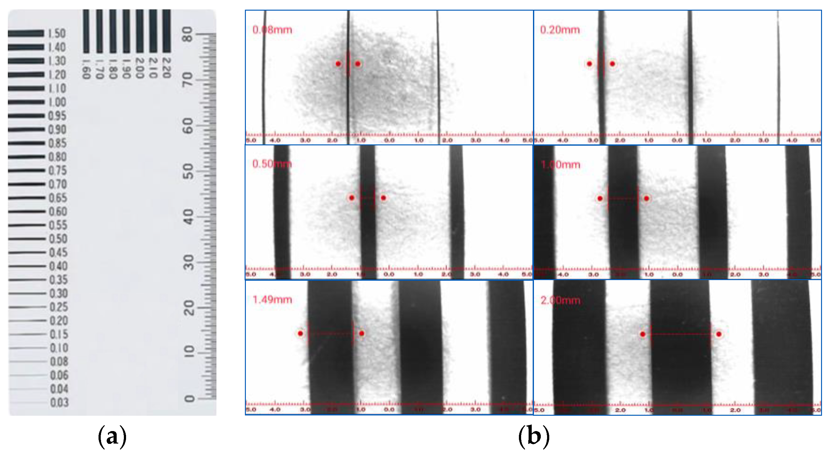
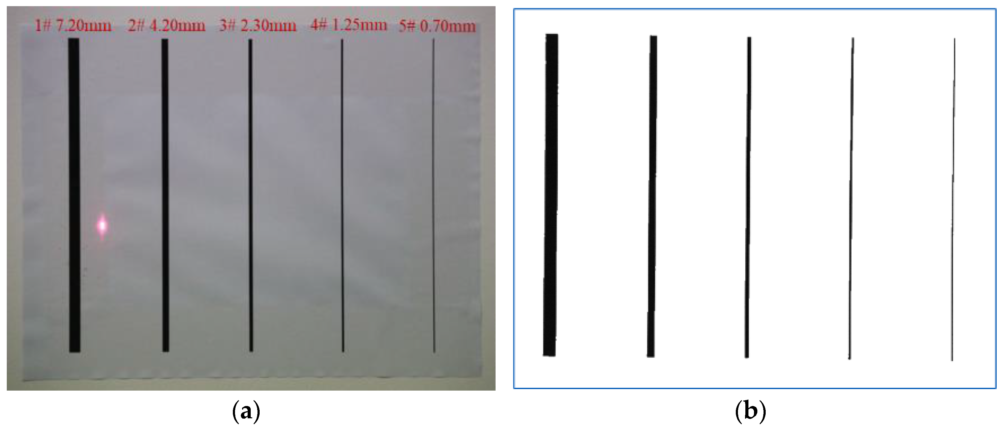
The measurement results for standard artificial cracks prove that the capturing angle and distance can significantly impact the accuracy; since the number of pixels the target occupies is reduced, the image resolution and unit pixel size would affect measurement results.
(2)
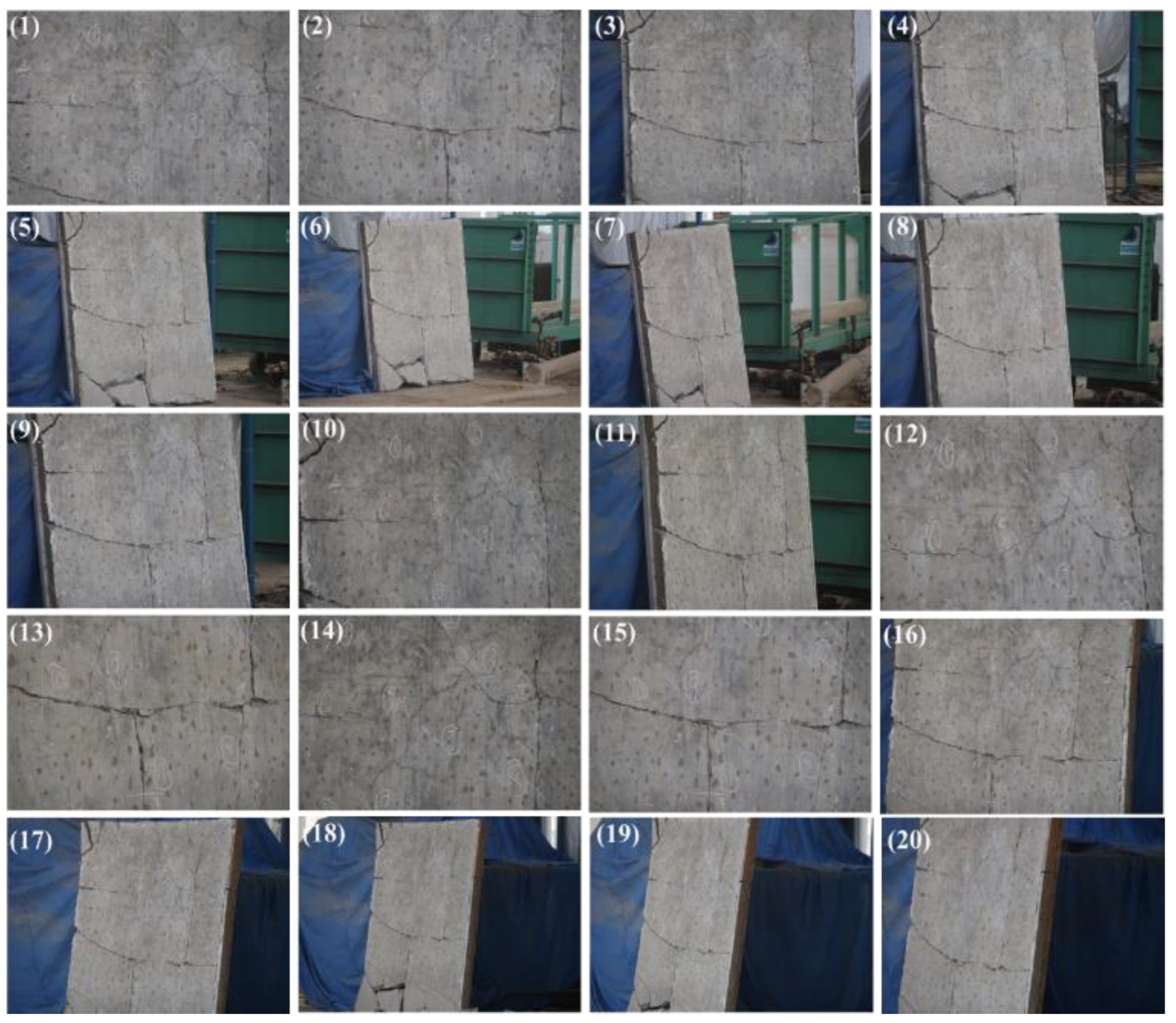
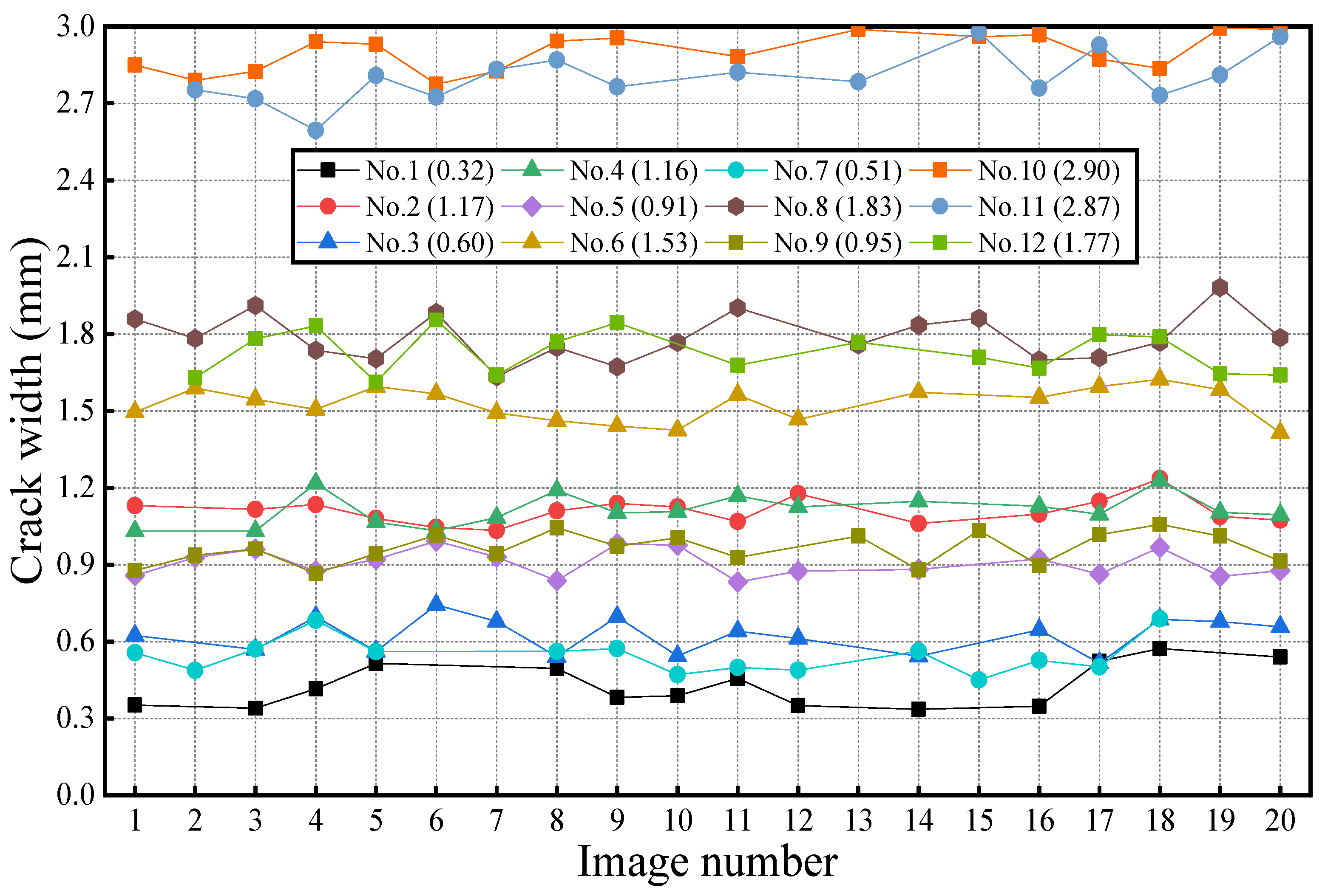
To further analyze the influencing factors of measurement accuracy, a concrete wall in the lab is adopted to measure the crack width. With capturing distances and horizontal angle changing from 5 to 20 m and −65° to 50°, 12 cracks widths are measured, and the average absolute error is less than 0.2 mm, which proves that the crack images taken from different angles and distances can be used to accurately calculate the crack width.
(3)
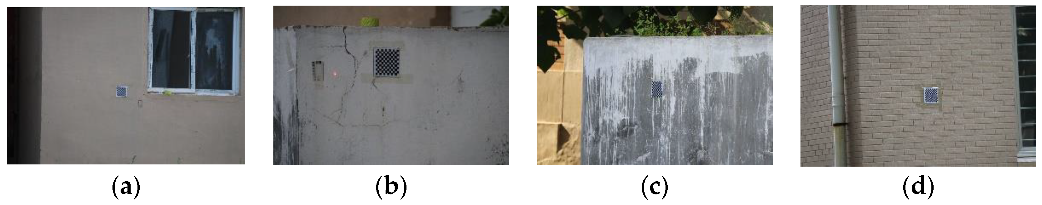
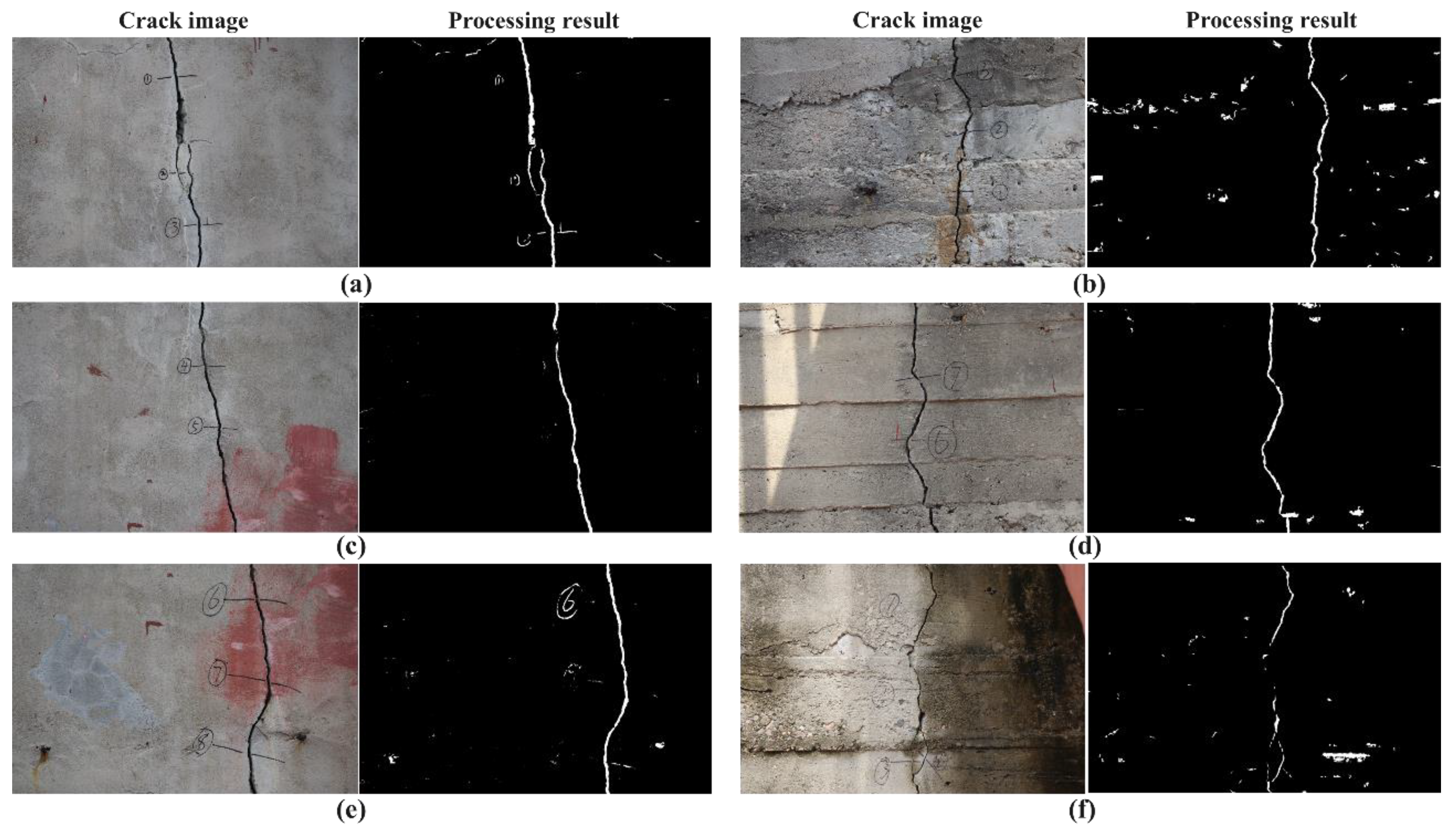
The performances of crack extraction with different backgrounds are also analyzed on several concrete walls. The maximum error occurs at the furthest position, which is calculated as −0.15 mm measured from 15.647 m. For cracks with a small captured angle, the relative error is less than 5%, which can prove the accuracy of the segmentation algorithm.
(4)
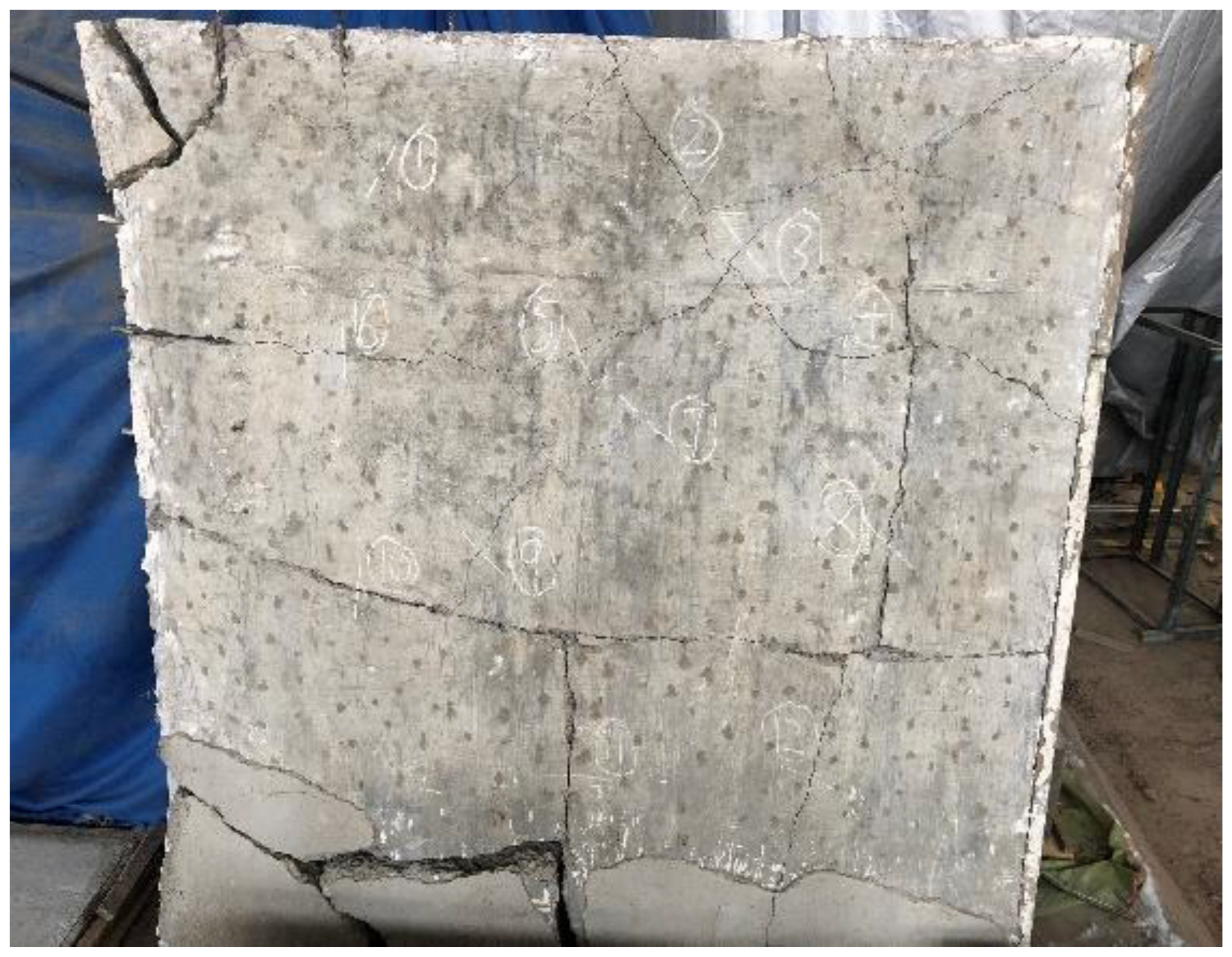
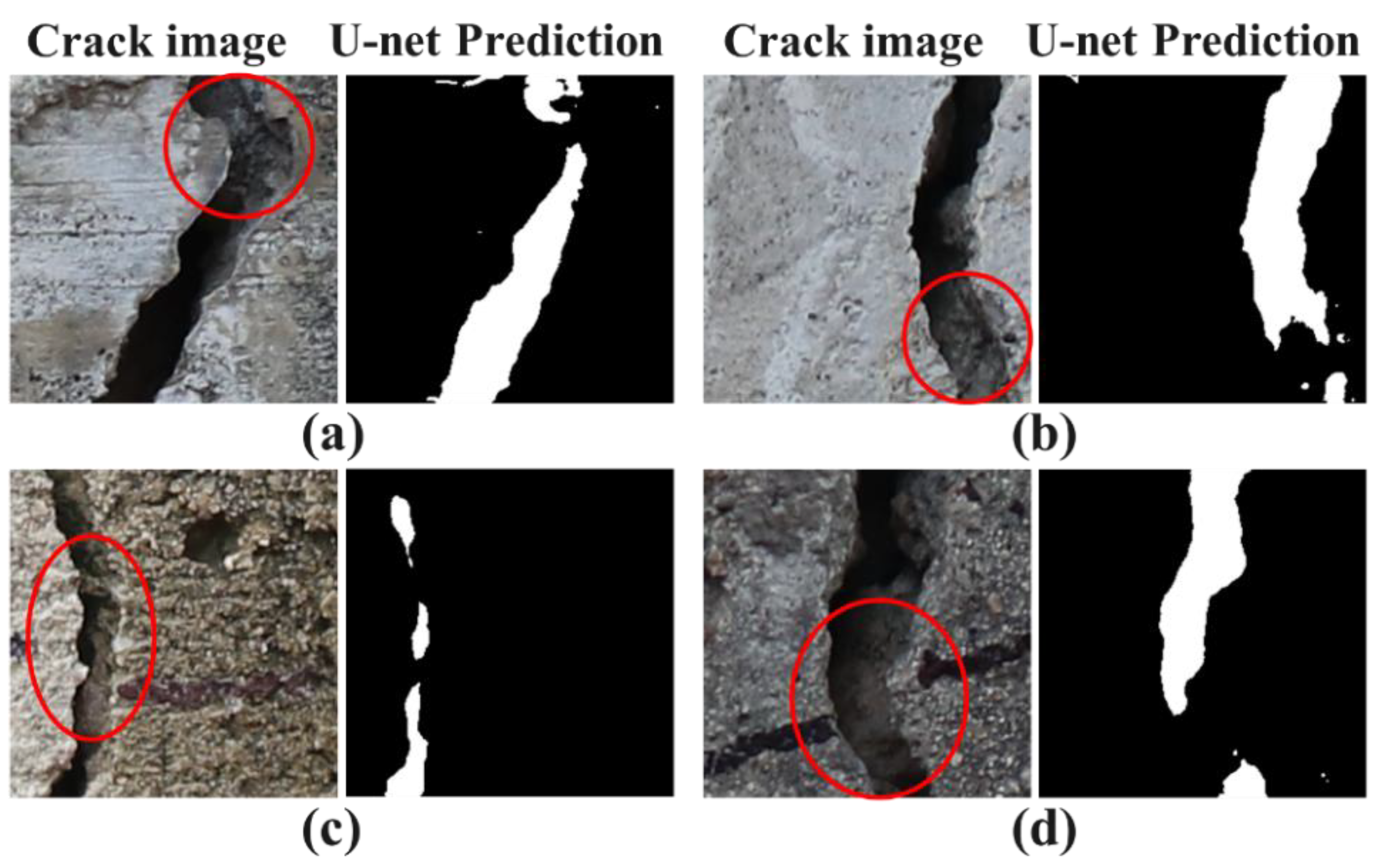
The measurement results on the concrete dam show that the protrusions that occur deep in the crack can affect the segmentation results, and the measurement error is increased. The measurement results are accurate and robust, which means the method presented in this paper has practical and scientific novelty.
(5)
In general, for the equipment used in this paper, the capturing angle should not be greater than 50°, and the photographing distance should be less than 30 m. The maximum measurement error obtained in this way is less than 0.3 mm. For concrete crack measurements, the performance of the camera and laser rangefinder combination system based on the improved U-net algorithm and Canny method is accurate and stable.

Author Contributions

Conceptualization, J.L. and F.K.; methodology, S.Z.; validation, F.K.; formal analysis, J.L. and F.K.; writing—review and editing, S.Z. and F.K. All authors have read and agreed to the published version of the manuscript.

Funding

This research was funded by National Key R & D Program of China grant number 2016YFC0401600 and 2017YFC0404900; National Natural Science Foundation of China grant number 51779035, 51769033 and 51979027, 52079022; Fundamental Research Funds for the Central Universities grant number DUT21TD106.

Institutional Review Board Statement

Not applicable.

Informed Consent Statement

Not applicable.

Conflicts of Interest

The authors declare no conflict of interest.

References

  1. Yang, Y.-S.; Wu, C.-L.; Hsu, T.T.; Yang, H.-C.; Lu, H.-J.; Chang, C.-C. Image analysis method for crack distribution and width estimation for reinforced concrete structures. Autom. Constr. 2018, 91, 120–132. [Google Scholar] [CrossRef]
  2. Liu, Y.F.; Nie, X.; Fan, J.S.; Liu, X.G. Image-based crack assessment of bridge piers using unmanned aerial vehicles and three-dimensional scene reconstruction. Comput. Civ. Infrastruct. Eng. 2020, 35, 511–529. [Google Scholar] [CrossRef]
  3. Amin, M.N.; Khan, K.; Ahmad, W.; Javed, M.F.; Qureshi, H.J.; Saleem, M.U.; Qadir, M.G.; Faraz, M.I. Compressive Strength Estimation of Geopolymer Composites through Novel Computational Approaches. Polymers 2022, 14, 2128. [Google Scholar] [CrossRef]
  4. Kang, F.; Li, J.; Zhao, S.; Wang, Y. Structural health monitoring of concrete dams using long-term air temperature for thermal effect simulation. Eng. Struct. 2019, 180, 642–653. [Google Scholar] [CrossRef]
  5. Chen, X.; Li, D.; Tang, X.; Liu, Y. A three-dimensional large-deformation random finite-element study of landslide runout considering spatially varying soil. Landslides 2021, 18, 3149–3162. [Google Scholar] [CrossRef]
  6. Gong, J.; Zou, D.; Kong, X.; Liu, J.; Qu, Y. An approach for simulating the interaction between soil and discontinuous structure with mixed interpolation interface. Eng. Struct. 2021, 237, 112035. [Google Scholar] [CrossRef]
  7. Canny, J. A Computational Approach to Edge Detection. IEEE Trans. Pattern Anal. Mach. Intell. 1986, 6, 679–698. [Google Scholar] [CrossRef]
  8. Asghar, R.; Javed, M.F.; Alrowais, R.; Khalil, A.; Mohamed, A.M.; Mohamed, A.; Vatin, N.I. Predicting the Lateral Load Carrying Capacity of Reinforced Concrete Rectangular Columns: Gene Expression Programming. Materials 2022, 15, 2673. [Google Scholar] [CrossRef]
  9. Cha, Y.-J.; Choi, W.; Büyüköztürk, O. Deep Learning-Based Crack Damage Detection Using Convolutional Neural Networks. Comput. Civ. Infrastruct. Eng. 2017, 32, 361–378. [Google Scholar] [CrossRef]
  10. Liu, Z.; Cao, Y.; Wang, Y.; Wang, W. Computer vision-based concrete crack detection using U-net fully convolutional networks. Autom. Constr. 2019, 104, 129–139. [Google Scholar] [CrossRef]
  11. Zhang, L.; Shen, J.; Zhu, B. A research on an improved Unet-based concrete crack detection algorithm. Struct. Health Monit. 2021, 20, 1864–1879. [Google Scholar] [CrossRef]
  12. Dung, C.V. Autonomous concrete crack detection using deep fully convolutional neural network. Autom. Constr. 2019, 99, 52–58. [Google Scholar] [CrossRef]
  13. Li, S.; Zhao, X.; Zhou, G. Automatic pixel-level multiple damage detection of concrete structure using fully convolutional network. Comput. Aided Civ. Infrastruct. Eng. 2019, 34, 616–634. [Google Scholar] [CrossRef]
  14. Wang, W.; Su, C. Semi-supervised semantic segmentation network for surface crack detection. Autom. Constr. 2021, 128, 103786. [Google Scholar] [CrossRef]
  15. Ronneberger, O.; Fischer, P.; Brox, T. U-Net: Convolutional networks for biomedical image segmentation. In Medical Image Computing and Computer-Assisted Intervention-MICCAI 2015, Proceedings of the International Conference on Medical Image Computing and Computer-Assisted Intervention, Munich, Germany, 5–9 October 2015; Springer: Cham, Switzerland, 2015; pp. 234–241. [Google Scholar] [CrossRef] [Green Version]
  16. Chen, K.; Reichard, G.; Xu, X.; Akanmu, A. Automated crack segmentation in close-range building façade inspection images using deep learning techniques. J. Build. Eng. 2021, 43, 102913. [Google Scholar] [CrossRef]
  17. Aslam, Y.; Santhi, N.; Ramasamy, N.; Ramar, K. Localization and segmentation of metal cracks using deep learning. J. Ambient Intell. Humaniz. Comput. 2021, 12, 4205–4213. [Google Scholar] [CrossRef]
  18. Sajedi, S.O.; Liang, X. Uncertainty-assisted deep vision structural health monitoring. Comput. Civ. Infrastruct. Eng. 2021, 36, 126–142. [Google Scholar] [CrossRef]
  19. Huyan, J.; Li, W.; Tighe, S.; Xu, Z.; Zhai, J. CrackU-net: A novel deep convolutional neural network for pixelwise pavement crack detection. Struct. Control Health Monit. 2020, 27, e2551. [Google Scholar] [CrossRef]
  20. Kong, S.-Y.; Fan, J.-S.; Liu, Y.-F.; Wei, X.-C.; Ma, X.-W. Automated crack assessment and quantitative growth monitoring. Comput. Aided. Civ. Infrastruct. Eng. 2021, 36, 656–674. [Google Scholar] [CrossRef]
  21. Jiang, S.; Zhang, J. Real-time crack assessment using deep neural networks with wall-climbing unmanned aerial system. Comput. Civ. Infrastruct. Eng. 2020, 35, 549–564. [Google Scholar] [CrossRef]
  22. Dias-Da-Costa, D.; Valença, J.; Júlio, E.; Araújo, H. Crack propagation monitoring using an image deformation approach. Struct. Control Health Monit. 2017, 24, e1973. [Google Scholar] [CrossRef] [Green Version]
  23. Zhao, S.; Kang, F.; Li, J.; Ma, C. Structural health monitoring and inspection of dams based on UAV photogrammetry with image 3D reconstruction. Autom. Constr. 2021, 130, 103832. [Google Scholar] [CrossRef]
  24. Perry, B.J.; Guo, Y. A portable three-component displacement measurement technique using an unmanned aerial vehicle (UAV) and computer vision: A proof of concept. Measurement 2021, 176, 109222. [Google Scholar] [CrossRef]
  25. Farahani, B.V.; Barros, F.; Sousa, P.J.; Cacciari, P.P.; Tavares, P.J.; Futai, M.M.; Moreira, P. A coupled 3D laser scanning and digital image correlation system for geometry acquisition and deformation monitoring of a railway tunnel. Tunn. Undergr. Space Technol. 2019, 91, 102995. [Google Scholar] [CrossRef]
  26. Yang, Y.; Sang, X.; Yang, S.; Hou, X.; Huang, Y. High-Precision Vision Sensor Method for Dam Surface Displacement Measurement. IEEE Sens. J. 2019, 19, 12475–12481. [Google Scholar] [CrossRef]
  27. Rezaie, A.; Achanta, R.; Godio, M.; Beyer, K. Comparison of crack segmentation using digital image correlation measurements and deep learning. Constr. Build. Mater. 2020, 261, 120474. [Google Scholar] [CrossRef]
  28. Ji, X.; Miao, Z.; Kromanis, R. Vision-based measurements of deformations and cracks for RC structure tests. Eng. Struct. 2020, 212, 110508. [Google Scholar] [CrossRef]
  29. Valença, J.; Júlio, E. MCrack-Dam: The scale-up of a method to assess cracks on concrete dams by image processing. The case study of Itaipu Dam, at the Brazil–Paraguay border. J. Civ. Struct. Health Monit. 2018, 8, 857–866. [Google Scholar] [CrossRef]
  30. Hao, X.-L.; Liang, H. A multi-class support vector machine real-time detection system for surface damage of conveyor belts based on visual saliency. Measurement 2019, 146, 125–132. [Google Scholar] [CrossRef]
  31. Jahanshahi, M.R.; Masri, S.F. Adaptive vision-based crack detection using 3D scene reconstruction for condition assessment of structures. Autom. Constr. 2012, 22, 567–576. [Google Scholar] [CrossRef]
  32. Yeum, C.M.; Dyke, S.J. Vision-Based Automated Crack Detection for Bridge Inspection. Comput. Civ. Infrastruct. Eng. 2015, 30, 759–770. [Google Scholar] [CrossRef]
  33. Wang, H.-F.; Zhai, L.; Huang, H.; Guan, L.-M.; Mu, K.-N.; Wang, G.-P. Measurement for cracks at the bottom of bridges based on tethered creeping unmanned aerial vehicle. Autom. Constr. 2020, 119, 103330. [Google Scholar] [CrossRef]
  34. Ali, R.; Chuah, J.H.; Talip, M.S.A.; Mokhtar, N.; Shoaib, M.A. Structural crack detection using deep convolutional neural networks. Autom. Constr. 2022, 133, 103989. [Google Scholar] [CrossRef]
  35. Finn, A.; Kumar, P.; Peters, S.; O’Hehir, J. Unsupervised spectral-spatial processing of drone imagery for identification of pine seedlings. ISPRS J. Photogramm. Remote Sens. 2022, 183, 363–388. [Google Scholar] [CrossRef]
  36. Kromanis, R.; Kripakaran, P. A multiple camera position approach for accurate displacement measurement using computer vision. J. Civ. Struct. Health Monit. 2021, 11, 661–678. [Google Scholar] [CrossRef]
  37. Jin, S.; Lee, S.E.; Hong, J.-W. A vision-based approach for autonomous crack width measurement with flexible kernel. Autom. Constr. 2020, 110, 103019. [Google Scholar] [CrossRef]
  38. Sudre, C.H.; Li, W.; Vercauteren, T.; Ourselin, S.; Jorge Cardoso, M. Generalised dice overlap as a deep learning loss function for highly unbalanced segmentations. In Deep Learning in Medical Image Analysis and Multimodal Learning for Clinical Decision Support; Springer: Cham, Switzerland, 2017; pp. 240–248. [Google Scholar] [CrossRef] [Green Version]
  39. Konig, J.; Jenkins, M.D.; Barrie, P.; Mannion, M.; Morison, G. A Convolutional Neural Network for Pavement Surface Crack Segmentation Using Residual Connections and Attention Gating. In Proceedings of the 2019 IEEE International Conference on Image Processing (ICIP), Taipei, Taiwan, 26 August 2019; pp. 1460–1464. [Google Scholar] [CrossRef] [Green Version]
  40. Adhikari, R.; Moselhi, O.; Bagchi, A. Image-based retrieval of concrete crack properties for bridge inspection. Autom. Constr. 2014, 39, 180–194. [Google Scholar] [CrossRef]
  41. Li, G.; Zhao, X.; Du, K.; Ru, F.; Zhang, Y. Recognition and evaluation of bridge cracks with modified active contour model and greedy search-based support vector machine. Autom. Constr. 2017, 78, 51–61. [Google Scholar] [CrossRef]
  42. Oh, J.-K.; Jang, G.; Oh, S.; Lee, J.H.; Yi, B.-J.; Moon, Y.S.; Lee, J.S.; Choi, Y. Bridge inspection robot system with machine vision. Autom. Constr. 2009, 18, 929–941. [Google Scholar] [CrossRef]
  43. Li, G.; He, S.; Ju, Y.; Du, K. Long-distance precision inspection method for bridge cracks with image processing. Autom. Constr. 2014, 41, 83–95. [Google Scholar] [CrossRef]
Figure 1. Imaging geometrical relationship of Gauss model.
Applsci 12 10651 g001
Figure 2. Problems of machine vision measurement methods. (a) Images of calibration board from side direction; (b) edges detected by Canny method, red circle is the discontinuous part.
Applsci 12 10651 g002
Figure 3. Crack measurement equipment composed of camera, laser rangefinder, laptop and tripod.
Applsci 12 10651 g003
Figure 4. Decomposition of unparallel plane into horizontal and vertical orientation.
Applsci 12 10651 g004
Figure 5. The geometric relationship between the combination of the camera and laser rangefinder and the target plane in clockwise direction: (a) horizontal length transformation; (b) vertical proportional relationship.
Applsci 12 10651 g005
Figure 6. The geometric relationship between the combination of the camera and laser rangefinder and the target plane in counter-clockwise direction: (a) horizontal length transformation; (b) vertical proportional relationship.
Applsci 12 10651 g006
Figure 7. Laser point center recognition: (a) original image of laser measuring point; (b) identified center by Hough transform.
Applsci 12 10651 g007
Figure 8. Architecture of U-net network for crack segmentation.
Applsci 12 10651 g008
Figure 9. The comparison between U-net extracted crack area and Canny edge detection: (a) example of crack refining process, where the gray values are the transition area; (b) influence of refinement on crack width measurement.
Applsci 12 10651 g009
Figure 10. Flowchart of image-based concrete crack detection and measurement.
Applsci 12 10651 g010
Figure 11. The HICHANCE-CK103 crack width measuring instrument for verification.
Applsci 12 10651 g011
Figure 12. Accuracy verification results of the adopted crack width measuring instrument: (a) crack scale board with several standard widths; (b) measurement results for standard widths.
Applsci 12 10651 g012
Figure 13. Calibration board for parameter determination: (a) training group; (b) testing group.
Applsci 12 10651 g013
Figure 14. Measurement value comparison before and after parameter correction.
Applsci 12 10651 g014
Figure 15. Accuracy and loss of the training and validation process of U-net: (a) accuracy; (b) loss.
Applsci 12 10651 g015
Figure 16. Precision, recall and F1 of U-net model performance on test dataset.
Applsci 12 10651 g016
Figure 17. Some grid size measuring scenarios: the distance, horizontal and vertical angle are (a) 20.2 m, 9°, 4°; (b) 8.7 m, 5°, 1°; (c) 15.4 m, −31°, −1°; (d) 18.2 m, 7°.
Applsci 12 10651 g017
Figure 18. Five artificial cracks: (a) original image with measured width; (b) segmentation results of the proposed method.
Applsci 12 10651 g018
Figure 19. Concrete wall with 12 naturally occurring cracks.
Applsci 12 10651 g019
Figure 20. Images of concrete wall photographed from different positions. The distances and the horizontal angles are (1) 8.6 m, 6°; (2) 8.7 m, 6°; (3) 13.0 m, 19°; (4) 14.7 m, 35°; (5) 16.8 m, 44°; (6) 20.4 m, 52°; (7) 17.7 m, 59°; (8) 14.3 m, 52°; (9) 12.0 m, 40°; (10) 8.2 m, 17°; (11) 10.7 m, 56°; (12) 5.6 m, 40°; (13) 5.7 m, 40°; (14) 7.1 m, 24°; (15) 7.2 m, 24°; (16) 11.5 m, −34°; (17) 14.2 m, −51°; (18) 17.6 m, −60°; (19) 15.1 m, −65°; (20) 11.1 m, −64°.
Applsci 12 10651 g020
Figure 21. Examples of crack segmentation on concrete wall; the blue circle is the location of crack width measurement.
Applsci 12 10651 g021
Figure 22. Measurement results of each crack in each image, and the real widths of 12 cracks. Of these, crack no. 1 is not detected in image 6, image 7 and image 19; crack no. 7 is not detected in image 6, image 7, image 19 and image 20.
Applsci 12 10651 g022
Figure 23. Segmentation results of cracks in outfield captured from different positions. (a) clear background, (b) dark background, (c) blurred boundaries, (d) bright background, (e) high contrast, (f) several cracks.
Applsci 12 10651 g023
Figure 24. Cracks on the dam pier: (a) panorama of the pier, where the red circle is the position of cracks; (b) crack with clear concrete background; (c) crack with wet and blurred background.
Applsci 12 10651 g024
Figure 25. Cracks on concrete dam pier with different background and segmentation results. (a) narrow crack, (b) artificial mark interference, (c) boundaries refinement, (d) blurry boundaries, (e) accurate segmentation, (f) artificial mark interference, (g) blurry boundaries, (h) boundaries refinement.
Applsci 12 10651 g025
Figure 26. Original image of the captured crack and the processed result. (a) crack No.1 to No.3 on simple background, (b) crack with lots of noises, (c) crack No.4 and No.5 on simple background, (d) crack on uneven plane, (e) crack No.6 to No.8 on simple background, (f) crack on complex background.
Applsci 12 10651 g026
Figure 27. The interference of the protrusion deep in the crack on the accuracy of dam crack segmentation. (a) segmentation discontinuity, red circle is the protrusion position; (b) segmentation error, red circle is the different protrusion style; (c) missing part of crack segmentation, red circle is the continuous protrusion; (d) protrusion similar to concrete surface, red circle is the protrusion position.
Applsci 12 10651 g027
Table 1. Comparison between measuring systems optimized by two objective parameters.
System CorrectionAEmean (cm)RMSE (cm)
Values without correction parameters0.05380.0687
Values with correction parameters0.00740.0097
Values of test group0.00620.0085
Table 2. Performance of U-net model for concrete crack segmentation.
DatasetPrecision Recall F1
Training 0.9160 0.9224 0.9181
Validation 0.9152 0.9171 0.9147
Testing 0.9016 0.9164 0.9075
Table 3. Measurements on the grid size of the calibration board.
NoParametersGrid Size and Error
Distance U (m)Horizontal θhVertical θvAverage Measured (mm)Error (mm)
120.22610.0780.078
28.74410.0830.083
315.498−31°−1°9.784−0.216
418.22610.0760.076
519.167−13°10.1180.118
630.11410°−3°9.817−0.183
722.68122°−4°10.2000.200
825.78210.1580.158
914.467−15°10.1090.109
109.265−6°19°10.1910.191
Table 4. Measurements results of five artificial cracks.
ParametersAverage Measurement Results (mm)Performance Criteria
Distance U (m)Horizontal
θh
Vertical
θv
1# (7.20)2# (4.20)3# (2.30)4# (1.250)5# (0.70)Average
Error
Maximum Error
9.77615°−3°7.3374.1582.3891.310.7840.0660.137
15.8667.2244.2992.4011.3450.7770.0790.101
20.3697.2094.2672.3261.2990.780.0460.08
10.490−11°−1°7.3274.3032.2761.3780.7560.0780.128
10.876−19°7.3484.0282.411.410.8160.072−0.172
Table 5. Evaluation of the 12 crack width values between measured in 20 images and real values (mm).
ItemStandardAverageAEmeanRMSE
Crack No. 10.320.354 0.147 0.183
Crack No. 21.171.110 0.069 0.077
Crack No. 30.600.626 0.064 0.071
Crack No. 41.161.115 0.064 0.074
Crack No. 50.910.908 0.046 0.051
Crack No. 61.531.527 0.057 0.064
Crack No. 70.510.431 0.152 0.244
Crack No. 81.831.789 0.085 0.098
Crack No. 90.950.9640.052 0.060
Crack No. 102.902.902 0.065 0.072
Crack No. 112.872.803 0.099 0.117
Crack No. 121.771.729 0.076 0.092
Table 6. The error of the proposed measurement system in 20 positions (mm).
ItemAbsolute Error
Average
Maximum
Absolute Error
R2
Image 10.0508 0.1290 0.9948
Image 20.0659 0.1400 0.9960
Image 30.0578 0.1520 0.9937
Image 40.0894 0.2750 0.9854
Image 50.0770 0.1950 0.9877
Image 60.1515 0.1450 0.9556
Image 70.1352 0.1960 0.9710
Image 80.0613 0.1760 0.9915
Image 90.0740 0.1580 0.9912
Image 100.0611 0.1050 0.9860
Image 110.0550 0.1370 0.9935
Image 120.0290 0.0630 0.9970
Image 130.0622 0.0890 0.9912
Image 140.0437 0.1090 0.9880
Image 150.0672 0.1080 0.9964
Image 160.0579 0.1310 0.9941
Image 170.0663 0.2040 0.9894
Image 180.0997 0.2530 0.9962
Image 190.1372 0.1520 0.9696
Image 200.1239 0.2200 0.9639
Table 7. Measurement results of six cracks on concrete wall.
NoStandard (mm)ParametersCrack Width and Error
Distance U (m)Horizontal θhVertical
θv
Measured (mm)Error (mm)Relative Value
Crack (a)0.7714.8510.778 −0.008−1.04%
Crack (b)1.306.18737°1.1690.13110.08%
Crack (c)2.747.34824°10°2.6590.0812.96%
Crack (d)3.0515.64725°2.9000.1504.92%
Crack (e)4.0714.59214°3.9650.1052.58%
Crack (f)2.1114.85120°2.0980.0120.57%
Table 8. Measurement results of cracks on the dam pier in Figure 22.
Image and Crack No.Standard (mm)ParametersCrack Width and Error
Distance U (m)Horizontal θhVertical
θv
Measured (mm)Error (mm)Relative Value
(a)-16.275.6456.0430.2273.62%
(a)-21.341.400−0.06−4.48%
(a)-35.986.028−0.048−0.80%
(b)-15.965.6756.192−0.232−3.89%
(b)-26.406.537−0.137−2.14%
(b)-34.85undetected--
(c)-45.405.5605.2620.1382.56%
(c)-55.064.9580.1022.02%
(d)-65.675.7765.4770.1933.40%
(d)-74.034.220−0.19−4.71%
(e)-65.164.9625.236−0.076−1.47%
(e)-75.355.397−0.047−0.88%
(e)-85.155.241−0.091−1.77%
(f)-13.735.5053.6730.0571.53%
(f)-23.47undetected--
(f)-30.870.902−0.032−3.68%
(f)-42.302.2660.0341.48%
Publisher’s Note: MDPI stays neutral with regard to jurisdictional claims in published maps and institutional affiliations.

